Download
1 / 7
70 likes | 151 Views
D etecting and Mapping Persistent Large-scale Turbidity Features in Chesapeake Bay Mainstem Waters – Phase I: Derivation of turbidity maxima from 670nm SeaWiFS reflectance data. V. Ransibrahmanakul 1 , D.E. Pirhalla 1 , T.T. Wynne 2 , A. Desch, L. Ojanen, and J.D. Christensen 1.

E N D
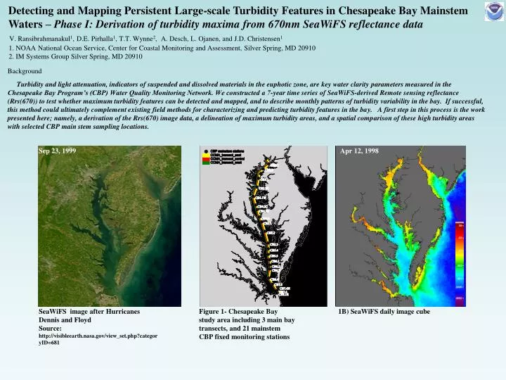
Detecting and Mapping Persistent Large-scale Turbidity Features in Chesapeake Bay Mainstem Waters – Phase I: Derivation of turbidity maxima from 670nm SeaWiFS reflectance data V. Ransibrahmanakul1, D.E. Pirhalla1, T.T. Wynne2, A. Desch, L. Ojanen, and J.D. Christensen1 1. NOAA National Ocean Service, Center for Coastal Monitoring and Assessment, Silver Spring, MD 20910 2. IM Systems Group Silver Spring, MD 20910 Background Turbidity and light attenuation, indicators of suspended and dissolved materials in the euphotic zone, are key water clarity parameters measured in the Chesapeake Bay Program’s (CBP) Water Quality Monitoring Network. We constructed a 7-year time series of SeaWiFS-derived Remote sensing reflectance (Rrs(670)) to test whether maximum turbidity features can be detected and mapped, and to describe monthly patterns of turbidity variability in the bay. If successful, this method could ultimately complement existing field methods for characterizing and predicting turbidity features in the bay. A first step in this process is the work presented here; namely, a derivation of the Rrs(670) image data, a delineation of maximum turbidity areas, and a spatial comparison of these high turbidity areas with selected CBP main stem sampling locations. Sep 23, 1999 Apr 12, 1998 SeaWiFS image after Hurricanes Dennis and Floyd Source: http://visibleearth.nasa.gov/view_set.php?categoryID=681 Figure 1- Chesapeake Bay study area including 3 main bay transects, and 21 mainstem CBP fixed monitoring stations 1B) SeaWiFS daily image cube
Methods For preliminary work, three main bay transects were used to extract instantaneous (daily) SeaWiFS Rrs(670) image data over the 7- year climatology. We used a moving 30-day median of Rrs(670) values to characterize variability of turbidity over time (Figure 2A,B,C). We then used counts of elevated Rrs(670) for each line number along the main bay transect for detection of bay turbidity maximum zone (TMZ). For comparison, we used counts of secchi depth data for 21CBP mainstem (CBx.x) fixed stations vs. Rrs(670) data, for the period (1997- 2004). We then calculated percent frequency of elevated turbidity by month for each transect line number to determine months of maximum turbidity derived from Rrs(670). Susquehanna River monthly discharge- cfs (Conowingo, MD gauge) 2A) Long term reflectance data for Center main stem transect 2B) Long term reflectance data for West main stem transect 2C) Long term reflectance data for East main stem transect Figure 2- Mainstem transects (A,B,C) (y-axis) were used to extract instantaneous pixel information from the SeaWiFS daily imagery. Color changes across time (x-axis) represent large-scale turbidity changes in the Chesapeake Bay mainstem. Transects consist of A) center main stem, B) east main stem and C) west main stem. This pixel-line array represents north-south turbidity variability over a 7-year period. Not surprisingly, as Susquehanna river discharge increases, Rrs increases in the northern Bay.
Results 3A) SeaWiFS-derived turbidity • Turbidity maxima (highest reflectance counts) occurred south of the Susquehanna River mouth- near Turkey Point (CB2.1)- line 13 (see arrow- Figure 3A) to near Poole’s Island (CB2.2)- line 37. • Spatial patterns of turbidity maxima, derived from 670 Rrs counts, appeared to be highly correlated with secchi depth (NTU adjusted) from long term fixed station monitoring. Turbidity Maximum Zone 3B) CBP fixed station secchi depth Turbidity Maximum Zone Figure 3- Comparison of SeaWiFS-derived turbidity vs. secchi depth from CBP fixed station monitoring. Figure 3A shows counts of Rrs(670) where reflectance values were greater than or equal to the 90th percentile (0.00492 /ster) of all values recorded (1997-2004). Counts were normalized by total number of samples per line. Figure 3B shows normalized counts of secchi depth >= .90 (0.7 m; 14.88 NTU) for the CBP stations shown (1997-2004). Conversion: NTU = ((1.45/secchi depth)-1)/0.072
January February March April May June July August September October November December Figure 4- Monthly comparison of reflectance counts >= 90th percentile of values. Shows months of occurrence of maximum turbidity for the period 1997-2004. Months of Occurrence • Highest turbidity occurred in December with a secondary peak in March and April, indicating seasonality of the Chesapeake Bay turbidity maxima zone.
Conclusions • Long term measures of turbidity derived from satellite may be used as a relative measure of turbidity conditions and trends in Chesapeake Bay mainstem waters. • Relative change (as opposed to absolute measures) of turbidity can be a highly useful alternative for measuring temporal and spatial variability of turbidity in Bay waters. • Key indicators of water quality, including turbidity are an important determinant of a healthy and productive Bay. The EPA’s Chesapeake Bay Program outlines specific water clarity criteria and levels of attainment necessary for sustainable plant communities. Turbidity products from satellite show strong potential for detecting and analyzing large-scale spatial and seasonal variability in turbidity. Months of Occurrence Figure 5- Monthly comparison of maximum turbidity for the period 1997-2004.Y-axis shows the percentage of reflectance counts >= 90th percentile of all values recorded. For more information contact: Varis Ransibrahmanakul varis.ransi@noaa.gov, or Douglas E. Pirhalla doug.pirhalla@noaa.gov 301-713-3028. NOAA/NOS Center for Coastal Monitoring and Assessment 1305 East West Hwy, SSMC-4, 9th fl. Silver Spring, MD 20910
Spatially and temporally correlate maximum turbidity values derived from Rrs 670 with each CBP fixed monitoring station (51 TOT)- Results may indicate the need for Bay- long sampling of light attenuation (Kd) indicators at specific wavelengths for validation. Develop climatology of average conditions along the mainstem transect- Important for longer term trend detection. Map “nearshore” vs. mid Bay temporal variability in turbidity signal associated with change in frequency and duration of flood events– concentrate on short and long term fluxes. Investigate how climate-induced changes in precipitation, Susquehanna River discharge, wind stress, and SLP would effect sediment inputs and turbidity in mainstem waters. Develop monitoring and assessment tools (eg. turbidity indices, forecasts) for comparing turbidity patterns month-month, season-season, year-year Next Steps xx) Long term normals of reflectance data for East main stem transect 2B) Long term reflectance data for East main stem transect Figure xx- Climatology of Rrs(670) for the period 1997-2004. Color changes across time (x-axis) represent large-scale turbidity changes in the Chesapeake Bay mainstem. Transect 2B) shows long term changes in Rrs(670) along east main stem.
Peak Susquehanna River discharge vs. elevated Turbidity derived from SeaWiFS 2006 June. 29, 2006 ~27 ~450,000 Jan. 10, 1998 Feb. 29, 2000 Apr. 12, 2001 May 15, 2002 Mar. 22, 2003 Sep. 19, 2004 Jan. 26, 1999 ?