Download
1 / 37
380 likes | 585 Views
Topic 16: Multicollinearity and Polynomial Regression. Outline. Multicollinearity Polynomial regression. An example (KNNL p256). The P-value for ANOVA F-test is <.0001 The P values for the individual regression coefficients are 0.1699, 0.2849, and 0.1896

E N D
Outline • Multicollinearity • Polynomial regression
An example (KNNL p256) • The P-value for ANOVA F-test is <.0001 • The P values for the individual regression coefficients are0.1699, 0.2849, and 0.1896 • None of these are near our standard significance level of 0.05 • What is the explanation? Multicollinearity!!!
Multicollinearity • Numerical analysis problem in that the matrix X΄X is close to singular and is therefore difficult to invert accurately • Statistical problem in that there is too much correlation among the explanatory variables and it is therefore difficult to determine the regression coefficients
Multicollinearity • Solve the statistical problem and the numerical problem will also be solved • We want to refine a model that currently has redundancy in the explanatory variables • Do this regardless if X΄X can be inverted without difficulty
Multicollinearity • Extreme cases can help us understand the problems caused by multicollinearity • Assume columns in X matrix were uncorrelated • Type I and Type II SS will be the same • The contribution of each explanatory variable to the model is the same whether or not the other explanatory variables are in the model
Multicollinearity • Suppose a linear combination of the explanatory variables is a constant • Example: X1 = X2→ X1-X2 = 0 • Example: 3X1-X2 = 5 • Example: SAT total = SATV + SATM • The Type II SS for the X’s involved will all be zero
An example: Part I Data a1; infile ‘../data/csdata.dat'; input id gpa hsm hss hse satm satv genderm1; Data a1; set a1; hs = (hsm+hse+hss)/3; Proc reg data=a1; model gpa= hsm hss hse hs; run;
Output • Something is wrong • dfM=3 but there are 4 X’s
Output NOTE: Model is not full rank. Least-squares solutions for the parameters are not unique. Some statistics will be misleading. A reported DF of 0 or B means that the estimate is biased.
Output NOTE: The following parameters have been set to 0, since the variables are a linear combination of other variables as shown. hs = 0.33333*hsm + 0.33333*hss + 0.33333*hse
Output In this extreme case, SAS does not consider hs in the model
Extent of multicollinearity • This example had one explanatory variable equal to a linear combination of other explanatory variables • This is the most extreme case of multicollinearity and is detected by statistical software because (X΄X) does not have an inverse • We are concerned with cases less extreme
An example: Part II *add a little noise to break up perfect linear association; Data a1; set a1; hs1 = hs + normal(612)*.05; Proc reg data=a1; model gpa= hsm hss hse hs1; run;
Output Model seems to be good here
Output • None of the predictors significant. • Look at the differences in Type I and II sums of squares • Sign of the coefficients?
Effects of multicollinearity • Regression coefficients are not well estimated and may be meaningless • Similarly for standard errors of these estimates • Type I SS and Type II SS will differ • R2 and predicted values are usually ok
Pairwise Correlations • Pairwise correlations can be used to check for “pairwise” collinearity • Recall KNNL p256 procreg data=a1 corr; model fat=skinfold thigh midarm; model midarm = skinfold thigh; run;
Pairwise Correlations • Cor(skinfold, thigh)=0.9238 • Cor(skinfold, midarm) = 0.4578 • Cor(thigh, midarm) = 0.0847 • Cor(midarm,skinfold+thigh) = 0.9952!!! • See p 284 for change in coeff values of skinfold and thigh depending on what variables are in the model
Polynomial regression • We can fit a quadratic, cubic, etc. relationship by defining squares, cubes, etc., of a single X in a data step and using them as additional explanatory variables • We can do this with more than one explanatory variable if needed • Issue: When we do this we generally create a multicollinearity problem
KNNL Example p300 • Response variable is the life (in cycles) of a power cell • Explanatory variables are • Charge rate (3 levels) • Temperature (3 levels) • This is a designed experiment
Input and check the data Data a1; infile ‘../data/ch08ta01.txt'; input cycles chrate temp; run; Proc print data=a1; run;
Create new variables and run the regression Data a1; set a1; chrate2=chrate*chrate; temp2=temp*temp; ct=chrate*temp; Proc reg data=a1; model cycles= chrate temp chrate2 temp2 ct; run;
Conclusion • Overall F significant, individual t’s not significant → multicollinearity problem • Look at the correlations (proc corr) • There are some very high correlations • r(chrate,chrate2) = 0.99103 • r(temp,temp2) = 0.98609 • Correlation between powers of a variable
A remedy • We can remove the correlation between explanatory variables and their powers by centering • Centering means that you subtract off the mean before squaring etc. • KNNL rescaled by standardizing (subtract the mean and divide by the standard deviation) but subtracting the mean is key here
A remedy • Use Proc Standard to center the explanatory variables • Recompute the squares, cubes, etc., using the centered variables • Rerun the regression analysis
Proc standard Data a2; set a1; schrate=chrate; stemp=temp; keep cycles schrate stemp; Proc standard data=a2 out=a3 mean=0 std=1; var schrate stemp; Proc print data=a3; run;
Recompute squares and cross product Data a3; set a3; schrate2=schrate*schrate; stemp2=stemp*stemp; sct=schrate*stemp;
Rerun regression Proc reg data=a3; model cycles=schrate stemp schrate2 stemp2 sct; run;
Output Exact same ANOVA table as before
Conclusion • Overall F significant • Individual t’s significant for chrate and temp • Appears linear model will suffice • Could do formal general linear test to assess this. (P-value is 0.5527)
Last slide • We went over KNNL 7.6 and 8.1. • We used programs Topic16.sas to generate the output for today