Download
1 / 12
130 likes | 512 Views
Unconstrained optimization. Gradient based algorithms Steepest descent Conjugate gradients Newton and quasi-Newton Population based algorithms Nelder Mead’s sequential simplex Stochastic algorithms. Unconstrained local minimization. The necessity for one dimensional searches

E N D
Unconstrained optimization • Gradient based algorithms • Steepest descent • Conjugate gradients • Newton and quasi-Newton • Population based algorithms • Nelder Mead’s sequential simplex • Stochastic algorithms
Unconstrained local minimization • The necessity for one dimensional searches • The most intuitive choice of skis the direction of steepest descent • This choice, however is very poor • Methods are based on the dictum that all functions of interest are locally quadratic
Conjugate gradients What are the unlabeled axes?
Newton and quasi-Newton methods • Newton • Quasi-Newton methods use successive evaluations of gradients to obtain approximation to Hessian or its inverse • Earliest was DFP, currently best known is BFGS • Like conjugate gradients guaranteed to converge in n steps or less for a quadratic function.
Matlabfminfunc X=FMINUNC(FUN,X0,OPTIONS) minimizes with the default optimization parameters replaced by values in the structure OPTIONS, an argumentcreated with the OPTIMSET function. See OPTIMSET for details. Used options are Display, TolX, TolFun, DerivativeCheck, Diagnostics, FunValCheck GradObj, HessPattern, Hessian, HessMult, HessUpdate, InitialHessType, InitialHessMatrix, MaxFunEvals, MaxIter,DiffMinChange and DiffMaxChange, LargeScale, MaxPCGIter,PrecondBandWidth, TolPCG, TypicalX.
Rosenbrock Banana function . Vanderplaats’sversion My version
Matlab output [x,fval,exitflag,output] = fminunc(@banana,[-1.2, 1]) Warning: Gradient must be provided for trust-region algorithm; using line-search algorithm instead. Local minimum found. Optimization completed because the size of the gradient is less than the default value of the function tolerance. x =1.0000 1.0000 fval =2.8336e-011 exitflag =1 output = iterations: 36, funcCount: 138 algorithm: 'medium-scale: Quasi-Newton line search‘ How would we reduce the number of iterations?
Sequential Simplex Method (section 4.2.1) • In n dimensional space start with n+1 particles at vertices of a regular (e.g., equilateral) simplex. • Reflect worst point about c.g. • Read about expansion and contraction
Matlab commands global z2 >> global yg >> global z1 >> global count >> count =1; >> options=optimset('MaxFunEvals',20) [x,fval] = fminsearch(@banana,[-1.2, 1],options) function [y]=banana(x) global z1 global z2 global yg global count y=100*(x(2)-x(1)^2)^2+(1-x(1))^2; z1(count)=x(1); z2(count)=x(2); yg(count)=y; count=count+1; >> mat=[z1;z2;yg] mat = Columns 1 through 8 -1.200 -1.260 -1.200 -1.140 -1.080 -1.080 -1.020 -0.960 1.000 1.000 1.050 1.050 1.075 1.125 1.1875 1.150 24.20 39.64 20.05 10.81 5.16 4.498 6.244 9.058 Columns 9 through 16 -1.020 -1.020 -1.065 -1.125 -1.046 -1.031 -1.007 -1.013 1.125 1.175 1.100 1.100 1.119 1.094 1.078 1.113 4.796 5.892 4.381 7.259 4.245 4.218 4.441 4.813
1.09 1.08 5.16 1.07 10.81 1.06 20.05 1.05 1.04 1.03 1.02 24,2 1.01 39.6 1 -1.26 -1.24 -1.22 -1.2 -1.18 -1.16 -1.14 -1.12 -1.1 -1.08 -1.06 fminsearch Banana function .
Completed search [x,fval,exitflag,output] = fminsearch(@banana,[-1.2, 1]) x =1.0000 1.0000 fval =8.1777e-010 exitflag =1 output = iterations: 85 funcCount: 159 algorithm: 'Nelder-Mead simplex direct search‘ Why is the number of iterations large compared to function evaluations (36 and 138 for fminunc)?