Download
1 / 49
490 likes | 599 Views
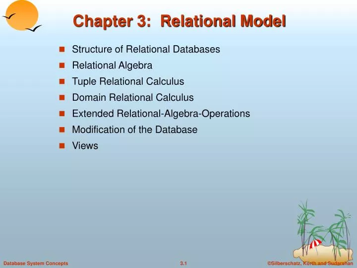
Chapter 3: Relational Model. Structure of Relational Databases Relational Algebra Tuple Relational Calculus Domain Relational Calculus Extended Relational-Algebra-Operations Modification of the Database Views. Example of a Relation. Basic Structure.

E N D
Chapter 3: Relational Model • Structure of Relational Databases • Relational Algebra • Tuple Relational Calculus • Domain Relational Calculus • Extended Relational-Algebra-Operations • Modification of the Database • Views
Basic Structure • Formally, given sets D1, D2, …. Dn a relation r is a subset of D1 x D2 x … x DnThus a relation is a set of n-tuples (a1, a2, …, an) where ai Di • Example: if customer-name = {Jones, Smith, Curry, Lindsay}customer-street = {Main, North, Park}customer-city = {Harrison, Rye, Pittsfield}Then r = { (Jones, Main, Harrison), (Smith, North, Rye), (Curry, North, Rye), (Lindsay, Park, Pittsfield)} is a relation over customer-name x customer-street x customer-city
Attribute Types • Each attribute of a relation has a name • The set of allowed values for each attribute is called the domain of the attribute • Attribute values are (normally) required to be atomic, that is, indivisible • E.g. multivalued attribute values are not atomic • E.g. composite attribute values are not atomic • The special value null is a member of every domain • The null value causes complications in the definition of many operations • we shall ignore the effect of null values in our main presentation and consider their effect later
Relation Schema • A1, A2, …, Anare attributes • R = (A1, A2, …, An ) is a relation schema E.g. Customer-schema = (customer-name, customer-street, customer-city) • r(R) is a relation on the relation schema R E.g. customer (Customer-schema)
Relation Instance • The current values (relation instance) of a relation are specified by a table • An element t of r is a tuple, represented by a row in a table attributes customer-name customer-street customer-city Jones Smith Curry Lindsay Main North North Park Harrison Rye Rye Pittsfield tuples customer
Database • A database consists of multiple relations • Information about an enterprise is broken up into parts, with each relation storing one part of the information E.g.: account : stores information about accountsdepositor : stores information about which customer owns which account customer : stores information about customers • Storing all information as a single relation such as bank(account-number, balance, customer-name, ..)results in • repetition of information (e.g. two customers own an account) • the need for null values (e.g. represent a customer without an account) • Normalization theory (Chapter 7) deals with how to design relational schemas
Keys • Let K R • K is a superkeyof R if values for K are sufficient to identify a unique tuple of each possible relation r(R) by “possible r” we mean a relation r that could exist in the enterprise we are modeling.Example: {customer-name, customer-street} and {customer-name} are both superkeys of Customer, if no two customers can possibly have the same name. • K is a candidate key if K is minimalExample: {customer-name} is a candidate key for Customer, since it is a superkey {assuming no two customers can possibly have the same name), and no subset of it is a superkey.
Determining Keys from E-R Sets • Strong entity set. The primary key of the entity set becomes the primary key of the relation. • Weak entity set. The primary key of the relation consists of the union of the primary key of the strong entity set and the discriminator of the weak entity set. • Relationship set. The union of the primary keys of the related entity sets becomes a super key of the relation. • For binary many-to-one relationship sets, the primary key of the “many” entity set becomes the relation’s primary key. • For one-to-one relationship sets, the relation’s primary key can be that of either entity set. • For many-to-many relationship sets, the union of the primary keys becomes the relation’s primary key
Query Languages • Language in which user requests information from the database. • Categories of languages • procedural • non-procedural • “Pure” languages: • Relational Algebra • Tuple Relational Calculus • Domain Relational Calculus • Pure languages form underlying basis of query languages that people use.
Relational Algebra • Procedural language • Six basic operators • select • project • union • set difference • Cartesian product • rename • The operators take two or more relations as inputs and give a new relation as a result.
Select Operation – Example A B C D • Relation r 1 5 12 23 7 7 3 10 • A=B ^ D > 5(r) A B C D 1 23 7 10
Select Operation • Notation: p(r) • p is called the selection predicate • Defined as: p(r) = {t | t rand p(t)} Where p is a formula in propositional calculus consisting of terms connected by : (and), (or), (not)Each term is one of: <attribute> op <attribute> or <constant> where op is one of: =, , >, . <. • Example of selection:branch-name=“Perryridge”(account)
Project Operation – Example • Relation r: A B C 10 20 30 40 1 1 1 2 A C A C • A,C (r) 1 1 1 2 1 1 2 =
Project Operation • Notation:A1, A2, …, Ak (r) where A1, A2 are attribute names and r is a relation name. • The result is defined as the relation of k columns obtained by erasing the columns that are not listed • Duplicate rows removed from result, since relations are sets • E.g. To eliminate the branch-name attribute of accountaccount-number, balance (account)
Union Operation – Example • Relations r, s: A B A B 1 2 1 2 3 s r r s: A B 1 2 1 3
Union Operation • Notation: r s • Defined as: r s = {t | t r or t s} • For r s to be valid. 1. r,s must have the same arity (same number of attributes) 2. The attribute domains must be compatible (e.g., 2nd column of r deals with the same type of values as does the 2nd column of s) • E.g. to find all customers with either an account or a loancustomer-name (depositor) customer-name (borrower)
Set Difference Operation – Example • Relations r, s: A B A B 1 2 1 2 3 s r r – s: A B 1 1
Set Difference Operation • Notation r – s • Defined as: r – s = {t | t rand t s} • Set differences must be taken between compatible relations. • r and s must have the same arity • attribute domains of r and s must be compatible
Cartesian-Product Operation-Example A B C D E Relations r, s: 1 2 10 10 20 10 a a b b r s r xs: A B C D E 1 1 1 1 2 2 2 2 10 19 20 10 10 10 20 10 a a b b a a b b
Cartesian-Product Operation • Notation r x s • Defined as: r x s = {t q | t r and q s} • Assume that attributes of r(R) and s(S) are disjoint. (That is, R S = ). • If attributes of r(R) and s(S) are not disjoint, then renaming must be used.
Composition of Operations • Can build expressions using multiple operations • Example: A=C(r x s) • r x s • A=C(r x s) A B C D E 1 1 1 1 2 2 2 2 10 19 20 10 10 10 20 10 a a b b a a b b A B C D E 10 20 20 a a b 1 2 2
Banking Example branch (branch-name, branch-city, assets) customer (customer-name, customer-street, customer-only) account (account-number, branch-name, balance) loan (loan-number, branch-name, amount) depositor (customer-name, account-number) borrower (customer-name, loan-number)
Example Queries • Find all loans of over $1200 amount> 1200 (loan) • Find the loan number for each loan of an amount greater than $1200 loan-number (amount> 1200 (loan))
Example Queries • Find the names of all customers who have a loan, an account, or both, from the bank customer-name (borrower) customer-name (depositor) • Find the names of all customers who have a loan and an account at bank. customer-name (borrower) customer-name (depositor)
Example Queries • Find the names of all customers who have a loan at the Perryridge branch. customer-name (branch-name=“Perryridge” (borrower.loan-number = loan.loan-number(borrower x loan))) • Find the names of all customers who have a loan at the Perryridge branch but do not have an account at any branch of the bank. customer-name (branch-name = “Perryridge” (borrower.loan-number = loan.loan-number(borrower x loan))) – customer-name(depositor)
Example Queries • Find the names of all customers who have a loan at the Perryridge branch. • Query 1customer-name(branch-name = “Perryridge” (borrower.loan-number = loan.loan-number(borrower x loan))) Query 2 customer-name(loan.loan-number = borrower.loan-number( (branch-name = “Perryridge”(loan)) x borrower) )
Example Queries Find the largest account balance • Rename account relation as d • The query is: balance(account) - account.balance (account.balance < d.balance(account x rd (account)))
Additional Operations We define additional operations that do not add any power to the relational algebra, but that simplify common queries. • Set intersection • Natural join • Division • Assignment
Set-Intersection Operation - Example • Relation r, s: • r s A B A B 1 2 1 2 3 r s A B 2
Natural-Join Operation • Notation: r s • Let r and s be relations on schemas R and S respectively.The result is a relation on schema R S which is obtained by considering each pair of tuples tr from r and ts from s. • If tr and ts have the same value on each of the attributes in RS, a tuple t is added to the result, where • t has the same value as tr on r • t has the same value as ts on s • Example: R = (A, B, C, D) S = (E, B, D) • Result schema = (A, B, C, D, E) • rs is defined as: r.A, r.B, r.C, r.D, s.E (r.B = s.B r.D = s.D (r x s))
r s Natural Join Operation – Example • Relations r, s: B D E A B C D 1 3 1 2 3 a a a b b 1 2 4 1 2 a a b a b r s A B C D E 1 1 1 1 2 a a a a b
Example Queries • Find all customers who have an account from at least the “Downtown” and the Uptown” branches. • Query 1 CN(BN=“Downtown”(depositoraccount)) CN(BN=“Uptown”(depositoraccount)) where CN denotes customer-name and BN denotes branch-name. • Query 2 customer-name, branch-name(depositoraccount) temp(branch-name) ({(“Downtown”), (“Uptown”)})
Example Queries • Find all customers who have an account at all branches located in Brooklyn city.customer-name, branch-name(depositoraccount) branch-name(branch-city = “Brooklyn”(branch))
Extended Relational-Algebra-Operations • Generalized Projection • Outer Join • Aggregate Functions
Aggregate Functions and Operations • Aggregation function takes a collection of values and returns a single value as a result. avg: average valuemin: minimum valuemax: maximum valuesum: sum of valuescount: number of values • Aggregate operation in relational algebra G1, G2, …, GngF1( A1), F2( A2),…, Fn( An)(E) • E is any relational-algebra expression • G1, G2 …, Gn is a list of attributes on which to group (can be empty) • Each Fiis an aggregate function • Each Aiis an attribute name
Aggregate Operation – Example • Relation r: A B C 7 7 3 10 sum-C gsum(c)(r) 27
Aggregate Operation – Example • Relation account grouped by branch-name: branch-name account-number balance Perryridge Perryridge Brighton Brighton Redwood A-102 A-201 A-217 A-215 A-222 400 900 750 750 700 branch-nameg sum(balance) (account) branch-name balance Perryridge Brighton Redwood 1300 1500 700
Aggregate Functions (Cont.) • Result of aggregation does not have a name • Can use rename operation to give it a name • For convenience, we permit renaming as part of aggregate operation branch-nameg sum(balance) as sum-balance (account)
Outer Join • An extension of the join operation that avoids loss of information. • Computes the join and then adds tuples form one relation that does not match tuples in the other relation to the result of the join. • Uses null values: • null signifies that the value is unknown or does not exist • All comparisons involving null are (roughly speaking) false by definition. • Will study precise meaning of comparisons with nulls later
Outer Join – Example • Relation loan branch-name loan-number amount Downtown Redwood Perryridge L-170 L-230 L-260 3000 4000 1700 • Relation borrower customer-name loan-number Jones Smith Hayes L-170 L-230 L-155
loan-number branch-name amount customer-name L-170 L-230 Downtown Redwood 3000 4000 Jones Smith Outer Join – Example • Inner Joinloan Borrower • Left Outer Join loan borrower loan-number branch-name amount customer-name L-170 L-230 L-260 Downtown Redwood Perryridge 3000 4000 1700 Jones Smith null
Outer Join – Example • Right Outer Join loanborrower loan-number branch-name amount customer-name L-170 L-230 L-155 Downtown Redwood null 3000 4000 null Jones Smith Hayes • Full Outer Join loan borrower loan-number branch-name amount customer-name L-170 L-230 L-260 L-155 Downtown Redwood Perryridge null 3000 4000 1700 null Jones Smith null Hayes
Null Values • It is possible for tuples to have a null value, denoted by null, for some of their attributes • null signifies an unknown value or that a value does not exist. • The result of any arithmetic expression involving null is null. • Aggregate functions simply ignore null values • Is an arbitrary decision. Could have returned null as result instead. • We follow the semantics of SQL in its handling of null values • For duplicate elimination and grouping, null is treated like any other value, and two nulls are assumed to be the same • Alternative: assume each null is different from each other • Both are arbitrary decisions, so we simply follow SQL
Null Values • Comparisons with null values return the special truth value unknown • If false was used instead of unknown, then not (A < 5) would not be equivalent to A >= 5 • Three-valued logic using the truth value unknown: • OR: (unknownortrue) = true, (unknownorfalse) = unknown (unknown or unknown) = unknown • AND: (true and unknown) = unknown, (false and unknown) = false, (unknown and unknown) = unknown • NOT: (not unknown) = unknown • In SQL “P is unknown” evaluates to true if predicate P evaluates to unknown • Result of select predicate is treated as false if it evaluates to unknown


![Chapter 3: Relational Model and Relational Algebra & Calculus ( [S] Chp . 2 and 5 )](https://cdn2.slideserve.com/4283663/chapter-3-relational-model-and-relational-algebra-calculus-s-chp-2-and-5-dt.jpg)