Download
1 / 40
400 likes | 610 Views
Acoustic Monitoring with the Beaufort Shelf Cabled Observatory. Peter Mikhalevsky Acoustic and Marine Systems Operation SAIC, Arlington, VA Cabled Observatory Workshop Barrow, Alaska Feb. 7-8, 2005. Acoustics in Arctic Observatories. Acoustic Remote Sensing

E N D
Acoustic Monitoring with the Beaufort Shelf Cabled Observatory Peter Mikhalevsky Acoustic and Marine Systems Operation SAIC, Arlington, VA Cabled Observatory Workshop Barrow, Alaska Feb. 7-8, 2005
Acoustics in Arctic Observatories • Acoustic Remote Sensing • Acoustic Thermometry and Tomography • Acoustic Halinometry • Acoustic Digital Current Profilers • Upward looking Ice Profiling Sonar • Multi-beam and side scan bathymetry and bottom profiling from AUV’s • Acoustic backscatter for biologics, effluents • Ambient Noise Monitoring • Marine mammals (bowhead whales) • Ice noise (correlated with thickness) • Seismics • Manmade noise, seismic surveys, drilling • Acoustic Communications • Data Telemetry and Network Control • Subsurface Navigation
Acoustic Remote Sensing Speed of sound is a function of water temperature and velocity and these can be derived from travel time measurements • Acoustic Thermometry • Average temperature and integral or average heat content along the propagation path between source and receiver, scale is function of source-receiver separation. • Arctic Ocean uniquely suited for acoustic thermometry due to good coupling of acoustic modes and major Arctic water masses
Acoustic Remote Sensing • Transport monitoring with acoustics • Use reciprocal transmissions to obtain projection of average transport along the propagation path • Two paths at different angles resolve current direction and speed • Combination of transport and heat measurements can provide heat flux • Acoustic Tomography • Use many intersecting paths to obtain spatial resolution and circulation, scale function of path density
Acoustic Remote Sensing: Examples • Convection Studies • Greenland Sea 1988-1989 • Mediterranean Sea 1991-1992, THETIS I • Transport Studies • Gibraltar 1996 • Basin Scale Studies – heat content • Mediterranean Sea 1994, THETIS II • North Pacific 1996-1999, 2002-?, ATOC • Arctic Ocean, 1994, 1998-1999, ACOUS Dushaw, et al.,”Observing the Ocean in the 2000’s: A Strategy for the Role of Acoustic Tomography in Ocean Climate Observation” in Observing the Oceans in the 21st Century, GODAE Project Office
Transport Monitoring in the Straits of Gibraltar Acoustic measurements black Curve, current meters red Send, et al., Deep Sea Res., 2002
Monitoring Temperature in the Western Mediterranean Acoustic measurement of average temperature 0-2000m ~30 m°C uncertainty Send, et al., Nature,1997
Arctic Climate Observations using Underwater Sound (ACOUS) • US/Russia bilateral program started in 1992 • Use acoustic thermometry to measure Arctic Ocean temperature and heat content • Feasibility exp. in 1994 showed strong coupling between travel times and AIW temp., observed basin scale AIW warming (~.4 °C avg. max) • Source installed in Oct. 1998 with transmissions every 4 days to receive array in Lincoln Sea (array recovered in Spring 2001) • Reception of source signals at APLIS ice camp in April 1999 showed continued warming in AIW consistent with SCICEX CTD’s (~.5°C avg. max)
Acoustic Remote Sensing in the Arctic MAJOR ARCTIC OCEAN WATER MASSES ARE WELL SAMPLED BYACOUSTIC MODES/RAYS Mikhalevsky, “Arctic Acoustics”, in Encyclopedia of Ocean Sciences, 2001
MODAL ARRIVAL PATTERN 1962 BEAUFORT SEA 20 Hz MODAL ARRIVAL PATTERN 1994 TRANS-ARCTIC PROPAGATION EXPERIMENT Mode 2 arrival ~ 2 secs earlier than model based on climatology STABLE ACOUSTIC PROPAGATION in the ARCTIC OCEAN
ACOUS - LINCOLN SEA EXPERIMENT ACOUS SOURCE – Franz Victoria StraitACOUS RECEIVE ARRAY - Lincoln Sea106, 20 min transmissions every four days Oct. 10, 1998 to Dec. 8, 1999
ACOUS SOURCE Deployed OCT. 1998 ACOUS VLA Deployed OCT. 1998 Recovered MAR. 2001
TEMPERATURE, SOUND SPEED and MODAL GROUP VELOCITIES Mode 1 speeds up
DIFFERENCE IN ARRIVAL TIME OF MODE 1 and MODE 2 + 0.3°C OVER 300 KM OF THE PATH SCICEX 99 10/10/1998 12/8/1999
Modeled sections consistent with acoustic data Temperature section using profiles from early 1990’s perturbed to fit “cooler” part of acoustic record Temperature section using profiles from late 1990’s perturbed to fit late 1999 “warm” part of acoustic record
ACOUS- LINCOLN SEA
Synoptic long term monitoring of sea ice Received acoustic energy on Lincoln Sea array o Filtered long period component A seasonal component can be clearly seen in the acoustic data o Modeled seasonal cycle* *D.A. Rothrock et.al., GRL,v.26(23), 1999
TEMPERATURE SECTIONS FROM SCICEX 1995, 1998, AND 1999 ACROSS THE ARCTIC BASIN WITH CORRESPONDING BATHYMETRY. WARMING IN THE ATLANTIC LAYER IS EVIDENT IN TOPOGRAPHICALLY GUIDED EXTENSIONS OF THE ATLANTIC WATER CIRCULATION.
SCICEX CTD SECTIONS AVERAGE TEMPERATURE OVER RANGE and DEPTH BETWEEN 0°C ISOTHERMS: 1995 - .421°C 1998 - .478°C 1999 - .488°C
Section AverageTemp. vs Travel Timerms fit error ~ 9 m°C Linear dependence on travel time of mode 2 (*) and Mode 3 (o) Integral Heat Content rms error ~ 7x10¹⁰ kJ/m 5 yr increase of ~1012 kJ/m over 2269 km path is 2.8 W/m2 heat flux
ACOUSTIC REMOTE SENSING Technical Requirements • Temperature and Heat content • Good clock for absolute travel time measurements, rubidium standard 1-8 ms/yr • Acoustic pulse travel time measurement precision of .5 ms demonstrated in TAP 1994 • Signal in Arctic from 1994-1999 for mode 2 (AIW temperature) was ~.4 secs/yr • Acoustic source and receiver technology very mature • Power requirements for basin scale observations ~250 watts acoustic power, ACOUS source ~50% efficiency, 20 min transmission ~.17 kWh
ACOUSTIC REMOTE SENSING CAPABILITIES in the ARCTIC • UNDER RESEARCH • Combine transport and temp. measurements for heat flux thru Fram Straits etc. • Average sea ice thickness and roughness over several hundreds of kms • Average thermocline layer depth over several hundreds of kms • Acoustic halinometry: changes in salinity and thickness of cold halocline layer
Acoustic Remote Sensing: Advantages • Permits rapid and repeated measurements over large ocean areas (3000 kt ship!) ie. basin scales for climate oriented studies • Measures the average properties between the moorings, “extends” coverage of field, the data grows as the product of the number of source and receiver moorings • Makes possible monitoring in regions where mooring installation/maintenance/recovery is difficult, eg. Arctic, Gulf Stream, Gibralter, Fram Strait, Bering Strait, etc.
ARCTIC REGIONAL UNDERSEA OBSERVATORY for RESEARCH and ANALYSIS AURORA VISION FOR EULERIAN ARCTIC MOORING GRID BASIN & STRAITS Exact number, layout and mooring design determined by multidisciplinary requirements Build in stages, Barrow Cabled Observatory, SEARCH, and build on experience from MARS and NEPTUNE International participation with cable terminations in Svalbard, Greenland, and Russia (as well as US and Canada) will greatly reduce undersea cable costs with cost sharing for system installation and operation
Acoustic monitoring: bowhead whales • Well documented that acoustic listening provides more accurate count than visual methods • Possibility to identify and track particular individuals • Current methods involve establishing ice camps and deploying hydrophones through the ice • Temporary, must be re-established, spring migration only • Subject to weather and ice conditions • Difficult to establish and maintain long baselines • Can drift out of optimal locations • Cabled observatory with field of distributed hydrophones or several distributed hydrophone arrays • Permanent presence, spring and fall migration • Available during all weather conditions year-round • Optimal sensor locations can be established and maintained
RECOMMENDATIONS • Integrated acoustic systems and sensors needed for observatory planning and design (http://www.oce.uri.edu/ao/IASOO) • Manage frequency spectrum, passive and active • Exploit same signals and sources/receivers for tomography, data telemetry and control, and navigation • Control noise environment (sources, pumps, AUV’s, etc.) • Impact on marine habitat and acoustic systems performance • Undertake detailed cost study for cable-based mooring undersea Arctic Ocean observing system and develop integrated plan leveraging existing and proposed programs like SEARCH, Neptune and the NSF Ocean Observatories Initiative
Consensus StatementOCEANOBS 1999 Conference* “In terms of the scientific approach to sampling the full depth of the ocean, globally, acoustic tomography… provides long-path, integral (low wavenumber) measurements of thermal variations to complement those from Argo and satellite altimetry.” “The Conference concluded that acoustic tomography did represent a potentially valuable approach and that, initially, it should be implemented in the Arctic…” *Koblinsky and Smith eds.,”Observing the Oceans in the 21st Century”
Temperature vertical average vs range Heat Content vertical average vs range Mode 2 Group Velocity EWG Climatology and SCICEX 95, 98, 99, 00
Acoustic Remote Sensing Implementation • Addition of acoustic hydrophones to moorings during the design phase costs ~$6K/phone for cabled moorings, and ~$26K/phone for autonomous moorings (on board data storage and rubidium clock required for latter), 4-8 phones per mooring required • Acoustic sources cost $300-500K depending on whether cabled or autonomous