Download
1 / 46
470 likes | 671 Views
Determining Type and Number of Automated Guided Vehicles Required in a System. Dr. David Sinreich Faculty of Industrial Engineering and Management Technion - Israel Institute of Technology. This presentation can’t be reproduced without the author’s permission.

E N D
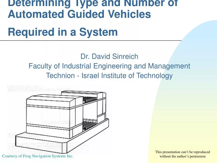
Determining Type and Number of Automated Guided Vehicles Required in a System Dr. David Sinreich Faculty of Industrial Engineering and Management Technion - Israel Institute of Technology This presentation can’t be reproduced without the author’s permission Courtesy of Frog Navigation Systems Inc.
Number of AGVs Flow Path Network WIP level Unit Load P/D Stations Control System IntroductionFactors which impact the system performance System’s Throughput and Lead Time
Number of AGVs Flow Path Network Unit Load P/D Stations IntroductionFactors which impact the required number of vehicles One of the most important factors which determine the performance level of a material handling system is the number of material handling devices operating in the system • The number of vehicles required so the system can operate efficiently is influenced by the unit load size and the flow path network and the location of P/D stations • The number of required vehicles has to be evaluated considering both economic and operational aspects
Unit load SizeThe impact on the vehicles Job orders arriving to the shop floor are divided into transferable unit loads, this division has a dual effect • The larger each unit load is the less transfers per time unit are required (reduced transfer capacity), hence less vehicles are needed to support these transfers • Based on the type and size (weight and volume) of the unit load transferred a vehicle type has to be chosen • The larger the unit load is the more expensive each vehicle will be • The opposite is also true smaller unit loads means a more vehicles are needed
cost Payload capacity Fleet size Unit load size Unit load size Unit load SizeThe impact on total cost of the system The larger the unit loads the more expensive the vehicles are due to the larger payloads required Total cost AGV cost inventory cost Container cost Cost/item moved Courtesy of Egbelu 1993
Flow Path NetworkThe impact on the vehicles The flow path network is made up of flow paths and intersections both of which have a direct impact on the time is takes a vehicle to complete its mission - delivering unit loads between pick-up and delivery stations flow paths intersections Long flow paths More intersections en route Proportional increase in flow time Potential increase in time delays Transfer capacity increase Transfer capacity increase More vehicles More vehicles The opposite is also true
P/D Station LocationThe impact on the vehicles The pick-up and delivery station location has a direct impact on the blocking, interference and time delays, vehicles encounter en route Locating P/D stations next to busy intersections and on track More blocking, interference and time delays Transfer capacity increase More vehicles Locating P/D stations away from busy intersections and off track Less vehicles
Vehicle CalculationBasic formula Required Transfer Capacity (Time) Number Vehicles = Planning Horizon (Time)
Vehicle CalculationThe states the vehicle can be in Idle moving or waiting While on assignment the vehicles may be: Empty Travel to pick-up station Blockedat any stage Loadinga unit load ChargingBatteries Loaded Travelto delivery station Unloadingthe unit load Idle time + Empty Travel time + Loading time + Loaded Travel time + Unloading time + Blocked time + Chargingtime = RequiredVehicle’s Transfer Capacity
Vehicle CalculationClassifying the different states The time duration the vehicle spends in any of the different states can be calculated in some cases and estimated in other cases States that their time duration can be calculated States that their time duration has to be estimated • Loading • Unloading • Loaded Travel • Idle • Empty Travel • Blocked • Charging
1 2 3 .. j 1 2 3 .. j 1 - f12 f13 .. f1j 1 - d12 d13 .. d1j 2 f21 - f23 .. f2j 2 d21 - d23 .. d2j : : : - .. : : : - .. i fi1 fi2 fi3 .. fij i di1 di2 di3 .. dij Vehicle CalculationFlow and distance matrices The time spent loading/unloading and traveling loaded can be calculated based on the From-To flow matrix and the Distance matrix between the pick-up and delivery stations of the different workcenters From-To matrix Distance matrix From pick-up station i to delivery station j Total number of transfer operations Total number of load and unload operations
Vehicle CalculationLoaded travel time and load/unload time calculations Let us define the following system parameters tL - Loading operation time tU - Unloading operation time V - Vehicle speed T - Time horizon Total time spent loading at pick-up stations (TL) Total time spent unloading at delivery stations (TU) Total loaded flow distance between workcenters Total loaded flow time (TLT)
Vehicle CalculationIdle, blocking, charging and empty travel time estimations • Idle, blocking and empty travel time are dependent on the rules, control methods and the dynamics of the system • Charging time is dependent on the type of batteries used/charging methods and assignments the vehicles perform • In order to estimate these times using simple methods estimation factors have been suggested e-vehicle’s efficiency estimation b-percentage of time the vehicle is blocked c - percentage of time the vehicle is idle tb - time estimation the vehicle spends charging -empty travel time estimation as a function of the loaded travel time
Vehicle CalculationSimple one dimensional methods • Methods are denoted as simple in the case the empty vehicle flow estimations are naive • These methods are denoted as one dimensional since predefined fixed unit load size and the flow path network are used, without considering an overall optimization • studies that fall under this category are: Maxwell and Muckstadt (1982), Egbelu (1987)
Vehicle CalculationSimple one dimensional methods (1) Simple Method 1 a constant as the empty travel function estimation (Egbelu 1987)
i Vehicle CalculationSimple one dimensional methods (2) Simple Method 2 empty travel estimation based on workcenter Net Flow (Egbelu 1987) fji fik : : NFi> 0- workcenter has a surplus of empty vehicles to export elsewhere NFi<0 - workcenter has a shortage of empty vehicle and needs to import NFi=0 - workcenter is self sufficient
ET2 Di Pi : : fji fik Vehicle CalculationSimple one dimensional methods (3) Empty travel distance between workcenters Empty travel distance between stations of the same workcenter * assuming average loaded flow distance = average empty flow distance
Vehicle CalculationSimple one dimensional methods (4) Simple Method 3 empty travel estimation using a transportation model (Maxwell & Muckstadt 1982) NFi > 0 NFi < 0 From delivery station i to pick-up station j This estimation serves as a lower bound to the actual empty travel Number of empty vehicles moving from delivery station i to pick-up station j
Vehicle CalculationComplex one dimensional methods • Methods are denoted as complex in the case empty vehicle flow estimations are more precise and use actual dispatching rules that are used on the shop floor such as FCFS and STT • studies that fall under this category are: Egbelu (1987), Bakkalbasi (1990), Malmborg (1991)
1 2 3 .. j 1 - f12 f13 .. f1j 2 f21 - f23 .. f2j : : : - .. : i fi1 fi2 fi3 .. fij Vehicle CalculationComplex one dimensional methods (1) Complex Method 1 empty travel estimation using FCFS* allocation rule (Egbelu 1987) pi - the probability that the next empty vehicle will be needed at pick-up station i pj - the probability that the next empty vehicle will be released at delivery station j *- First Come First Serve
1 2 3 .. j 1 2 3 .. j 1 - f12 f13 .. f1j 1 - g12 g13 .. g1j 2 f21 - f23 .. f2j 2 g21 - g23 .. g2j : : : - .. : : : : - .. : i fi1 fi2 fi3 .. fij i gi1 gi2 gi3 .. gij Vehicle CalculationComplex one dimensional methods (2) pij - probability that the empty vehicle that was assigned to travel to pick-up station i came from delivery station j gij - expected number of empty vehicle trips originating at delivery station j traveling to pick-up station i From delivery station j to pick-up station i
Vehicle CalculationMulti dimensional methods • Methods are denoted as multi dimensional in the case the vehicle calculation problem is integrated with other directly related problems such as unit load size determination and flow path design • studies that integrate vehicle calculation with flow path design are: Ashayeri (1989), • studies that integrate vehicle calculation with unit load size determination are: Mahadevan and Narendran (1992), Egbelu (1993) and Beamon and Deshpande (1998)
no lane from node i to node j one lane set up fromnode i to node j Vehicle Calculationmulti dimensional methods (1) Multi Dimensional Method 1 in conjunction with flow path design (Ashayeri 1989) Notation m - number of flow types fijk- number oftransfers required from node i to node j of flow type k NFik - net flow at node i of flow type k per hour Cpij - number of transfers allowed on a path from node i to n ode j per hour Wij - maximum number of flow path lanes allowed between nodes i and j Lij - lane installation cost from node i and j C - cost per vehicle including software and hardware
Vehicle Calculationmulti dimensional methods (2) Cost related to the number of vehicles required in the system Cost of the flow path network Maintaining the flow in the system Determining the number of flow path lanes required
Vehicle Calculationmulti dimensional methods (3) Multi Dimensional Method 2 in conjunction with the unit load size determination (Beamon and Deshpande 1998) Notation Akij - number of parts of type k that need to be transferred from station i to j Cp- capacity of each vehicle (parts) Lmax, Lmin - maximal allowed and minimal desired vehicle utilization N - number of vehicles required to operate the system Ukij - number of unit loads of part k need to be transferred from station i to j uk - size of unit load which contains parts of type k W(uk) - load unload time of unit loads as a function of the unit load size
Vehicle Calculationmulti dimensional methods (4) Maximizing parts being transferred within a pre-specified amount of time Determining number of transfers based on unit load size Limiting Transfer capacity of vehicle Limiting vehicle utilization Limiting unit load size based on transfer lots and vehicle capacity
What Is NextStatic and dynamic factors The required number of vehicles is effected by: • Static predetermined factors such as the number of transfers (unit load size), transfer distances, load/unload time and type of battery charging methods all which can be calculated or estimated in a reasonable accurate manner (as shown by the previous models) • Dynamic factors such as empty vehicle flow, dispatching rules, scheduling rules and mutual vehicle interference all which have a variable impact on the process The dynamic interference in general reduces the potential availability of vehicles and as a result reduces the vehicles fleet transfer capacity
What Is NextDrawbacks of analytical calculation methods • Since not all of the issues involved in the transport process can be modeled using analytical methods the dynamic factors are hard to predict and as a result vehicle calculations are not accurate enough • There is always a tradeoff between operational performance and economic aspects as a result determining the number of vehicles required in a system has to do with a sensitivity analysis and a decision making processes rather than a single calculated number
Throughput Number of vehicles Operational Versus Economic AspectsMutual vehicle interference Any addition of vehicles beyond this point reduces system performance due to mutual interference Max system throughput In the case the loss in throughput is marginal compared to the reduction in the number of vehicles it may be an economic gain Time-in-System Reduced number of vehicles The same analysis is true for the job’s time-in-system Max number of vehicles
SimulationEvaluating the number of vehicles (1) • The conclusion of all of this is that all vehicle calculation and optimization methods discussed thus far only serve as a first estimator to a more comprehensive method to evaluate (not calculate) the required number of vehicles in a system • Simulation is the only method that can accurately predict the system’s performance when using a specific number of specific vehicles in the system • Tanchoco et al. (1987) compare CAN-Q a tool which is based on queuing theory with AGVSim a dedicated AGV simulation tool and reinforce the above conclusions
SimulationEvaluating the number of vehicles (2) Sinreich and Tanchoco (1992) quantify the system’s throughput performance as function of the number of vehicles in the system using an extensive simulation study. This function is used in conjunction with a multi-goal optimization formulation to evaluate the required number of vehicles based on a tradeoff between cost and throughput Notation Pk, qk - negative and positive deviation from goal k respectively Cveh- cost of automated vehicle Ccont - controller cost which includes hardware and software Cbat - cost of battery charging station Cfix - fixed cost of related to the design and installation of the guide path Nmax - maximum number of vehicles which can operate in the system
- weight associated with the relative importance of the positive and negative deviation of goal k SimulationEvaluating the number of vehicles (3) Notation Mc - maximum number of vehicles a single controller can accommodate Mb- maximum number of vehicles a single charger can accommodate Th - management’s target throughput C - management’s target system cost a1,a2 - functioncoefficients describing the system’s throughput performance
SimulationEvaluating the number of vehicles (4) Minimizing the positive and negative deviations from desired management’s goals Management’s cost goal Management’s throughput goal A concave function which represents the system’s throughput behavior
SimulationDecision tablesforevaluating the number of vehicles Based on this formulation and for a predetermined range of management goals, decision tables can be developed to be used to evaluate the required number of vehicles Management’s throughput goal Management’s cost goal Trade-off ratio (% to $) Suggested number of vehicles
80 60 80 P3 D4 60 4 60 P4 1 80 D3 110 110 3 5 70 70 P1 80 P2 D5 P5 20 60 80 D2 P6 90 2 6 70 70 D6 80 140 Numerical Example6 department manufacturing facility (1)
Numerical Example6 department manufacturing facility (2) Vehicle carrying capacity - 500 lb Tote weight - 10 lb Tote volume - 500 in3 Vehicle traveling speed - 150 ft/min Loading and unloading time - 30 seconds Average job’s interarrival rate - 24 minuets Planning horizon - 8 hours Battery charging during planning horizon - 30 minuets
Numerical Example6 department manufacturing facility (3) During the the planning horizon 8/0.4 = 20 will arrive with the following job mix: Job1 - 20x0.3=6, Job2 - 8, Job3 - 4 and Job4 - 2 Based on this information the From-To flow matrix can be calculated based on the physical facility the distance matrix can be determined
Numerical Example6 department manufacturing facility (4) From-To Flow matrix Distance matrix e = 0.85
Small To Medium Unit Load AGVs Courtesy of Rapistan Demag Corp. and Apogee
Fork AGVs Courtesy of BT Systems Inc. and Apogee
Pallet AGVs Courtesy of Rapistan Demag Corp.
Heavy Load AGVs Courtesy of Rapistan Demag Corp., Mentor AGVS Inc. and Frog Navigation Systems Inc.
Towing AGVs Courtesy of Rapistan Demag Corp., Apogee and Control Engineering Company
Assignment Dedicated AGVs Courtesy of Rapistan Demag Corp., Apogee, Control Engineering Company and Mentor AGVS Inc.
Work Platform AGVs Courtesy of BT Systems Inc.