Download
1 / 25
260 likes | 358 Views
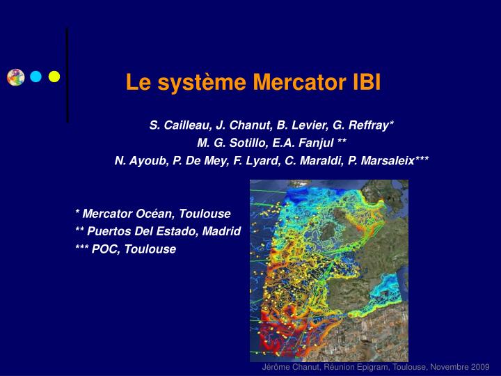
Le système Mercator IBI. S. Cailleau, J. Chanut, B. Levier, G. Reffray* M. G. Sotillo, E.A. Fanjul ** N. Ayoub, P. De Mey, F. Lyard, C. Maraldi, P. Marsaleix*** * Mercator Océan, Toulouse ** Puertos Del Estado, Madrid *** POC, Toulouse. Le contexte / les enjeux.

E N D
Le système Mercator IBI • S. Cailleau, J. Chanut, B. Levier, G. Reffray* • M. G. Sotillo, E.A. Fanjul ** • N. Ayoub, P. De Mey, F. Lyard, C. Maraldi, P. Marsaleix*** • * Mercator Océan, Toulouse • ** Puertos Del Estado, Madrid • *** POC, Toulouse
Le contexte / les enjeux • Une initiative nationale financée par le SHOM en 2006-2008 pour améliorer les performances des systèmes opérationels sur l’Atlantique Nord-Est . Complétée par un projet d’intercomparaison de NEMO sur le Golfe de Gascogne (Reffray et al, 2008) avec Mars, Symphonie et Hycom. • Poursuite des developments gràce à différents projets Européens (ECOOP, EASY). Participation active au dévelopement de NEMO pour les besoins spécifiques à la modélisation régionale. • MyOcean: Vers l’Intégration opérationnelle d’un système IBI, certifié, partagé entre Puertos et Toulouse en Avril 2011.
Mercator IBI technical description • NEMO 2.3 • Horizontal resolution: 1/36°, 2 km (1/12° for sensitivity studies) • z-coord + partial bottom cells (1m resolution near the surface) • Vertical mixing: 1.5 TKE (Gaspar et al. 1990)/ K-epsilon • Biharmonic momentum diffusion • Specific to IBI compared to basin scale models: • Explicit free surface with time splitting (rdt=150s, nn_baro= 50) • Quickest advection scheme for tracers • No explicit horizontal diffusion for tracers • Non-linear free surface (key_vvl) • 35 rivers implemented as lateral point sources (key_bdy) • Tidal potential • Open boundary schemes: 2d: characteristic method (Blayo and Debreu 2005). 3d: flow relaxation (30 pts, 1 day). • Open boundary data: “slow component” from 1/12° North Atlantic + tides from FES2004 + inverse barometer. Divergence/rotational conserving interpolations for slow component. • High frequency atmospheric forcing (3h). Atmospheric pressure gradient included. Spatially variable solar penetration length scales from ocean colour climatological observations.
Performances on ECMWF IBM super-computer • 1/36° grid (Memory ≈ 117 Go): equivalent to NATL12 • 792 sub-domains, 543 processors • 32% land points suppressed • CPU (elapsed) ≈ 50 min / week (c1a) • storage: 2 Go / output • 1/12° grid (Memory ≈ 13 Go): • 256 sub-domains, 192 processors • 25% land points suppressed • CPU (elapsed) ≈ 9 min / week • storage: 200 Mo / output
Modelling tides with NEMO:Move to non-linear, explicit free surface • Move from filtered, unsplitted free surface to mode-splitted free surface. Fast gravity waves resolved. • Non-linear free-surface: relax η<<H hypothesis. Update the vertical coordinate at each time step. Important for compound tidal waves, residual currents, internal waves induced mixing…
Comparison to insitu observations: Moving from 1/12° to 1/36° improves the statistics in general. 1/36° model outperforms TPXO 7.1 but still not as good as FES2004. NEATL36 FES2004 Non-linear, explicit free surface in NEMO NEATL36 FES2004
Non linear free surface MOG2D Linear free surface Impact of non-linear free surface: M4 tidal wave amplitude [m] and phase [°]
Non-linear, explicit free surface in NEMO Courants M2 Modèle vs obs. insitu
Non-linear, explicit free surface in NEMO Modèle vs vitesses M2 radar Rapport de validation disponible: cmaraldi@mercator-ocean.fr
Time splitting scheme update • Why ? • Actual time splitting scheme (Griffies et al, 2001) does not conserve tracers locally (because of modified continuity equation for stability reasons). Maybe acceptable for climate oriented simulations, but not for tidal applications on the shelf... • Replace existing scheme by ROMS UCLA generalized forward-backward (Shchepetkin and McWilliams, OM, 2005): conservative and cheaper ! Tests ok in NVTK double gyre configuration and in the North East Atlantic regional model. • Implies deep modification of the code structure (Tracers updated after dynamics...). Not compatible with implicit pressure gradient (key_hpgimp). • Coupling with the leapfrog time stepping for internal (3d) mode still does not ensure correct centering of forcing terms in barotropic equations.
> 2 psu ! New time splitting scheme supresses spurious freshwater along the coast.
Vertical mixing update • Generic length-scale equation model of Umlauf and Burchard (2003) implemented. Resolves two prognostic equations for turbulent kinetic energy and a generic length scale. Thanks to the latter, commonly used closures can be retrieved: k-ε, Mellor Yamada... • Study impact on tidal mixing fronts position, summertime SST bias, overflows
MODIS OPA HYCOM SYMP MARS Intercomparison experiments from Reffray et al, 2008
TKE k-ε k-ε - TKE Tidal mixing fronts: TKE vs k-ε SSTs May 2008 Excessive bottom boundary layer turbulent mixing with TKE
Reducing summertime SST bias? • Add climatological solar attenuation coefficients based on satellite kd490 data. • Should be accurate for type I water (turbidity=f[Chl]) ie not on the shelf ! Note that even for type I water different algorithms lead to more than substantial differences. • Recent parameterization for type II water (ie including absorption due to CDOM among others) based on IOPs could be tested (Lee et al, 2005, JGR). What about inter-annual variability ?
Clear water type vs variable attenuation (globcolour) +0.75°C Model too warm SST Bias OBS – MOD SST(MOD_var) – SST(MOD_typeI) June 2004
Globcolour Diff. relative % SEAWIF
May SST difference SEAWIF-GLOBCOLOUR • Recent parameterization for type II water (ie including absorption due to CDOM among others) based on IOPs could be tested (Lee et al, 2005, JGR). • What about inter-annual variability ?
Intégration pré-opérationnelle (Avril 2010) J0 J-7 J-14 J+14 Optimisation / Filtrage ? J+5 J+1 J+2 Scénarioopérationnel J+3
Intégration pré-opérationnelle Q1: Temps de convergence de la solution sur le plateau ?
Intégration pré-opérationnelle T=0 T=15 jours Q2: Convergence énergétique vs divergence vis à vis de la solution assimilée ? Quel impact sur la méso-échelle ? Q3: Réalité (vraisemblablement plutôt réalisme au sens statistique) des structures de submésoéchelle ? Utilisation de diagnostiques Lagrangiens ?