Download
1 / 17
180 likes | 375 Views
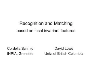
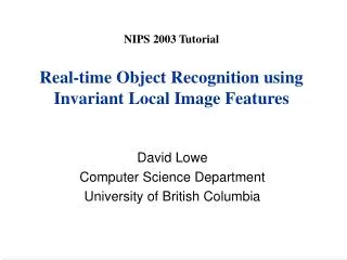
CVPR 2003 Tutorial Recognition and Matching Based on Local Invariant Features. David Lowe Computer Science Department University of British Columbia. Object Recognition. Definition: Identify an object and determine its pose and model parameters Commercial object recognition

E N D
CVPR 2003 TutorialRecognition and Matching Based on Local Invariant Features David Lowe Computer Science Department University of British Columbia
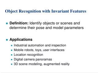
Object Recognition • Definition: Identify an object and determine its pose and model parameters • Commercial object recognition • Currently a $4 billion/year industry for inspection and assembly • Almost entirely based on template matching • Upcoming applications • Mobile robots, toys, user interfaces • Location recognition • Digital camera panoramas, 3D scene modeling
Invariant Local Features • Image content is transformed into local feature coordinates that are invariant to translation, rotation, scale, and other imaging parameters SIFT Features
Advantages of invariant local features • Locality: features are local, so robust to occlusion and clutter (no prior segmentation) • Distinctiveness: individual features can be matched to a large database of objects • Quantity: many features can be generated for even small objects • Efficiency: close to real-time performance • Extensibility: can easily be extended to wide range of differing feature types, with each adding robustness
Scale invariance Requires a method to repeatably select points in location and scale: • The only reasonable scale-space kernel is a Gaussian (Koenderink, 1984; Lindeberg, 1994) • An efficient choice is to detect peaks in the difference of Gaussian pyramid (Burt & Adelson, 1983; Crowley & Parker, 1984 – but examining more scales) • Difference-of-Gaussian with constant ratio of scales is a close approximation to Lindeberg’s scale-normalized Laplacian (can be shown from the heat diffusion equation)
Key point localization • Detect maxima and minima of difference-of-Gaussian in scale space • Fit a quadratic to surrounding values for sub-pixel and sub-scale interpolation (Brown & Lowe, 2002) • Taylor expansion around point: • Offset of extremum (use finite differences for derivatives):
Sampling frequency for scale More points are found as sampling frequency increases, but accuracy of matching decreases after 3 scales/octave
Sampling frequency for spatial domain • Need to determine number of pixels (samples) relative to smoothing • Image size is doubled to keep highest spatial frequencies
Select canonical orientation • Create histogram of local gradient directions computed at selected scale • Assign canonical orientation at peak of smoothed histogram • Each key specifies stable 2D coordinates (x, y, scale, orientation)
Example of keypoint detection Threshold on value at DOG peak and on ratio of principle curvatures (Harris approach) • (a) 233x189 image • (b) 832 DOG extrema • (c) 729 left after peak • value threshold • (d) 536 left after testing • ratio of principle • curvatures
Edelman, Intrator & Poggio (97) showed that complex cell outputs are better for 3D recognition than simple correlation Creating features stable to viewpoint change
Classification of rotated 3D models (Edelman 97): Complex cells: 94% vs simple cells: 35% Stability to viewpoint change
SIFT vector formation • Thresholded image gradients are sampled over 16x16 array of locations in scale space • Create array of orientation histograms • 8 orientations x 4x4 histogram array = 128 dimensions
Feature stability to noise • Match features after random change in image scale & orientation, with differing levels of image noise • Find nearest neighbor in database of 30,000 features
Feature stability to affine change • Match features after random change in image scale & orientation, with 2% image noise, and affine distortion • Find nearest neighbor in database of 30,000 features
Distinctiveness of features • Vary size of database of features, with 30 degree affine change, 2% image noise • Measure % correct for single nearest neighbor match