Download
1 / 27
270 likes | 502 Views
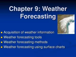
Weather Forecasting Chapter 9. Dr. Craig Clements SJSU Met 10. How to prepare a Weather Forecast. Acquisition of weather information Weather forecasting tools Weather forecasting methods

E N D
Weather Forecasting Chapter 9 Dr. Craig Clements SJSU Met 10
How to prepare a Weather Forecast • Acquisition of weather information • Weather forecasting tools • Weather forecasting methods • Forecasts provide information for the public (advisories). This information can be a critical safety issue, such as thunderstorms, fire weather conditions, etc.
Flags indicating advisories and warnings in maritime areas. Figure 1, p. 237
Doppler radar data from Melbourne, Florida, on March 25, 1992, during the time of a severe hailstorm that caused $60 million in damages in the Orlando area. In the table near the top of the display, the hail algorithm determined that there was 100 percent probability that the storm was producing hail and severe hail. The algorithm also estimated the maximum size of the hailstones to be greater than 3 inches. A forecaster can project the movement of the storm and adequately warn those areas in the immediate path of severe weather. Fig. 9-2, p. 238
A Meteogram illustrating predicted weather elements Fig. 9-3, p. 239
A sounding of air temperature, dew point, and winds. Fig. 9-4, p. 239
geostationary satellite The geostationary satellite moves through space at the same rate that the earth rotates, so it remains above a fixed spot on the equator and monitors one area constantly. Fig. 9-5, p. 240
Polar-orbiting satellites Polar-orbiting satellites scan from north to south, and on each successive orbit the satellite scans an area farther to the west. Fig. 9-6, p. 241
Generally, the lower the cloud, the warmer its top. Warm objects emit more infrared energy than do cold objects. Thus, an infrared satellite picture can distinguish warm, low (gray) clouds from cold, high (white) clouds
Three Satellite Products (tools) for the forecaster • Visible satellite images • Infrared images • Water vapor images
A visible image of the eastern Pacific Ocean Clouds in the visible image appear white Fig. 9-9a, p. 242
Infrared satellite image of the eastern Pacific Ocean Notice that the low clouds in the infrared image appear in various shades of gray Fig. 9-9b, p. 242
An enhanced infrared image Fig. 9-10, p. 243
Infrared water vapor image The darker areas represent dry air aloft; the brighter the gray, the more moist the air in the middle or upper troposphere. Bright white areas represent dense cirrus clouds or the tops of thunderstorms. The area in color represents the coldest cloud tops. The swirl of moisture off the West Coast represents a well-developed mid-latitude cyclonic storm. Fig. 9-11, p. 243
AWIPS computer work station provides various weather maps Fig. 9-1, p. 238
Numerical Weather Models A forecast chart is produced by computers solving the equations of motion and heat for the atmosphere. These charts are called prognostic charts of progs. These computer simulations solve the equations more quickly than can be done by hand. For example, to produce a 24-hr forecast chart for the Northern Hemisphere it requires hundreds of millions of mathematical calculations. It would take meteorologists working non-stop with hand calculators years to produce a single chart!
500-mb progs for 7 P.M. EST, July 12, 2006 — 48 hours into the future A resolution (grid spacing) of 12 km Fig. 9-12a, p. 245
500-mb progs for 7 P.M. EST, July 12, 2006 — 48 hours into the future GFS model with a resolution of 60 km Fig. 9-12b, p. 245
The 500-mb analysis for 7 P.M. EST, July 12, 2006 Fig. 9-13, p. 245
Ensemble 500-mb forecast chart for July 21, 2005 (48 hours into the future). The chart is constructed by running the model 15 different times, each time beginning with a slightly different initial condition. The blue lines represent the 5790-meter contour line; the red lines, the 5940-meter contour line; and the green line, the 500-mb 25-year average, called climatology. Fig. 9-14, p. 247
The 90-day outlook for (a) precipitation and (b) temperature for February, March, and April, 1999. Fig. 9-17, p. 251
A halo around the sun (or moon) means that rain is on the way. Fig. 9-18, p. 253