Download
1 / 25
250 likes | 418 Views
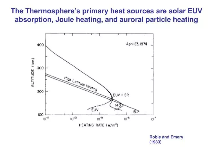
The Thermosphere’s primary heat sources are solar EUV absorption, Joule heating , and auroral particle heating. Roble and Emery (1983). Solar UV & EUV. photoelectron heating. photoionization. O 2 + h O + O. N 2 + h N + N. minor species diffusion N( 2 D) N( 4 S) NO.

E N D
The Thermosphere’s primary heat sources are solar EUV absorption, Joule heating, and auroral particle heating Roble and Emery (1983)
Solar UV & EUV photoelectron heating photoionization O2 + h O + O N2 + h N + N minor species diffusion N(2D) N(4S) NO electron and Ion energy equation ionosphere with O+ diffusion: O2+ N2+ NO+ N+ in PCE* major species diffusion O2 O and N2 nn nn nn Tn ni *photochemical equilibrium heating Ion/neutral chemistry neutral gas energy equation heating O recombination heating electron/ion/neutral collisions heating neutral-neutral chemistry
Electromagnetic Energy Flux KineticEnergy Flux Ionization hn e~ 20% e~ 80% Chemical Reactions Cascading e– Excitation e~ 5% Neutral Momentum Neutral Heating Ti Te e~ 50% Polar Energy Input to Thermospheric Heating
Simulations of Joule Heating and Thermosphere Density The global mean density variation computed from TIMEGCM for about 18 days in November 2004 (black line), together with the Joule heating derived from TIMEGCM (red line). A major storm on days 313-316, 2004 produced large density enhancements. Courtesy G. Crowley
SATELLITE DRAG AND THE EVOLUTION OF MODEL ATMOSPHERES The aerodynamic force is the force created by a spacecraft’s movement through a neutral density atmosphere. The force results from momentum exchange between the atmosphere and the spacecraft and can be decomposed into components of lift, drag, and side slip. The drag force is considered the most dominant force on low-earth orbiting spacecraft and serves to change the energy of the spacecraft through the work done by the drag force. This alters the period and semimajor axis of a spacecraft over time.
Through Kepler's laws, one can derive the rate of change of orbital period ( T ) in terms of the atmospheric density: where B = B-factor (ballistic coefficient) = rP = density at perigee = density s = satellite path Atmospheric Density determined by tracking the change of the orbital period From radar tracking, one can derive the atmospheric density (the more accurate the tracking, the shorter time required to determine density). Typical resolution is about 1 day below 200 km and 5 days at 500 km. (Much better with laser beacon, etc.)
The above procedure requires some knowledge about the variation of density with height. Given the equations defining the hydrostatic law, the chemical composition at some height, and an expression for the temperature profile shape (example: Bates Temperature Model), a density profile can be retrieved from the satellite observations. In practical applications of this method, if a reasonable initial first guess of the vertical structure is provided, an iterative procedure leads to an accurate determination that is independent of the initial guess. A set of "exospheric temperatures” emerges from this process.
Analyses of many satellite orbits led to the so-called "static diffusion models" developed by Jacchia and which form the basis of many operational drag models. These are based on a parameteric dependence of density on exospheric temperature. The derived exospheric temperatures (and the densities) reveal many of the variations typical of the thermosphere: annual, semiannual, solar activity, magnetic activity, diurnal, etc. (see following figures). DESPITE THE IMMENSE SUCCESS OF THESE MODELS AT THE TIME, THEY SUFFER FROM SOME FUNDAMENTAL LIMITATIONS: • The derived temperature is more of a 'virtual' temperature than 'real' (kinetic) temperature • Rocket measurements of O, O2 at the lower boundary are difficult to interpret (i.e., O recombines into O2 against walls of measuring device, meaning that O can be underestimated and O2 overestimated). • Wind-induced diffusion is also important, i.e., for [O]; The 'static diffusion' or 'hydrostatic' restriction is not amenable to addressing vertical transport (i.e., upwelling) or horizontal transport.
IN THE 1970'S, TWO DATA SETS BECAME AVAILABLE THAT ADDRESS THE PREVIOUSLY-MENTIONED LIMITATIONS FOR DRAG-BASED MODELS: • determinations of Tex from incoherent scatter radar measurements. • satellite mass spectrometer measurements of O, O2, N2, He, H, etc., and also measurements of Tex. (satellites like OGO-6, AE, and many others). HENCE LEADING TO THE: Mass Spectrometer Incoherent Scatter (MSIS) models of A. Hedin (NASA/GSFC). However, the MSIS models are not optimized with respect to satellite drag, and so have not been widely adopted for ephemeris computations in lieu of the Jacchia models. In principle, though, getting closer to the correct physics should lead to improved orbital predictions.
Some of the other models developed during the past 30 years EMPIRICAL http://ccmc.gsfc.nasa.gov/modelweb/ http://www.spenvis.oma.be/spenvis/ U.S. Standard 1962 Jacchia 1964 U.S. Standard Supplements, 1966 CIRA-1961, 1965 MSIS86, MSIS90, MSISE90 Jacchia-1971, 1977 CIRA-1986 NRLMSISE-00Jacchia-Bowman 2006 NUMERICAL/THEORETICAL MODELS University College London Thermosphere-Ionosphere Model (now Coupled Thermosphere-Ionosphere-Plasmasphere Model (CTIP) at CU/CIRES) NCAR Thermosphere-Ionosphere GCM TGCM TIGCM TIE-GCM TIME-GCM ASEN 5335 Aerospace Environments -- Upper Atmospheres
Correlation of density and temperature with long- term changes in solar activity.
Solar-Terrestrial Coupling Effects in the Thermosphere: New Perspectives from CHAMP and GRACE Accelerometer Measurements of Winds And Densities J. M. Forbes1, E.K. Sutton1, S. Bruinsma2, R. S. Nerem1 1Department of Aerospace Engineering Sciences, University of Colorado, Boulder, Colorado, USA 2Department of Terrestrial and Planetary Geodesy, CNES,Toulouse, France ASEN 5335 Aerospace Environments -- Drag & Re-entry
The CHAMP satellite was launched in July 2000 at 450 km altitude in a near-circular orbit with an inclination of 87.3° • The physical parameters of the CHAMP satellite are: • • Total Mass 522 kg • Height 0.750 m • • Length (with 4.044 m Boom) 8.333 m • Width 1.621 m • • Area to Mass Ratio 0.00138 m2kg-1
Non-gravitational forces acting • on the CHAMP and GRACE satellites • are measured in the in-track, • cross-track and radial directions • by the STAR accelerometer • Separation of accelerations due to mass density (in-track) or winds (cross-track and radial) require accurate knowledge of • spacecraft attitude • 3-dimensional modeling of the spacecraft surface (shape, drag coefficient, reflectivity, etc.) • accelerations due to thrusting • solar radiation pressure • Earth albedo radiation pressure STAR accelerometer by Onera
DMSP DMSP Only cross -track winds can be inferred CHAMP and GRACE offer new perspectives on thermosphere density response characterization: latitude, longitude, temporal and local time sampling Local time precession rate of CHAMP is about 24 hours/133 days ≈ 45 minutes November 20, 2003
Liu et al., JGR, 2005: “Global Distribution of the Thermospheric Mass Density Derived from CHAMP” Percent Differences from MSIS90 for Kp = 0-2 during 2002 > 50o Latitude Cusp region enhancement Pre-midnight/ midnight enhancement North-South asymmetry Co-location with field-aligned currents
~200 -300% ~200% EUV Flare ~50% Thermosphere Density Response to the October 29-31 2003 Storms from CHAMP Accelerometer Measurements (Sutton et al., JGR, 2005)
November 19-21 2003 Storm Density Structures at Scales > 1200 km: “Large-Scale” Waves ……. before _____ after (150-sec (~1200 km) running means applied to raw data)
~800 ms-1 April 2002 storm period % density difference from orbit average