Download
1 / 69
780 likes | 1.13k Views
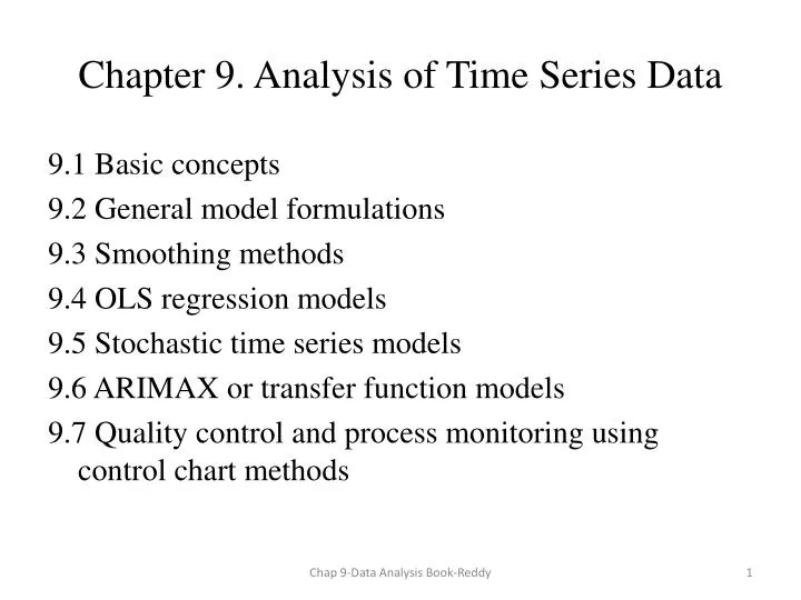
Chapter 9. Analysis of Time Series Data. 9.1 Basic concepts 9.2 General model formulations 9.3 Smoothing methods 9.4 OLS regression models 9.5 Stochastic time series models 9.6 ARIMAX or transfer function models 9.7 Quality control and process monitoring using control chart methods.

E N D
Chapter 9. Analysis of Time Series Data 9.1 Basic concepts 9.2 General model formulations 9.3 Smoothing methods 9.4 OLS regression models 9.5 Stochastic time series models 9.6 ARIMAX or transfer function models 9.7 Quality control and process monitoring using control chart methods Chap 9-Data Analysis Book-Reddy
9.1 Introduction • Time series data is not merely data collected over time. If this definition were true, then almost any data set would qualify as time series data. • There must be some sort of ordering , i.e. a relation between successive data observations. Successive observations in time-series data are not independent and their sequence needs to be maintained during the analysis. • Definition of time series data: A collection of numerical observations arranged in a natural order with each observation associated with a particular instant of time which provides the ordering • Practical way of ascertaining whether the data is to be treated as time series data or not, is to determine if the analysis results would change if the sequence of the data observations were to be scrambled. • The importance of time series analysis is that it provides insights and more accurate modeling and prediction to time series data than do classical statistical analysis because of the explicit manner of treating model residual Chap 9-Data Analysis Book-Reddy
Fig. 9.1 Daily peak and minimum hourly loads over several months for a large electric utility to illustrate the diurnal, the weekday/weekend and the seasonal fluctuations and trends. Chap 9-Data Analysis Book-Reddy
9.1.2 Terminology Chap 9-Data Analysis Book-Reddy
9.1.3. Basic behavior patterns • Constant process, • (b) linear trend, • (c) cyclic variation, • (d) impulse, • (e) step function, • (f) ramp Much of the challenge in time series analysis is distinguishing these basic behavior patterns when they occur in conjunction. The problem is compounded by the fact that processes may exhibit these patterns at different times. Fig.9.3. Different characteristics of time series (from Montgomery and Johnson 1976 by permission of McGraw-Hill) Chap 9-Data Analysis Book-Reddy
9.1.4 Illustrative Data Set Fig. 9.4 Time series data of electric power demand by quarter (Data from Table 9.1) Chap 9-Data Analysis Book-Reddy
9.2 General Model Formulation How does one model the behavior of the data shown in Example 9.1.1 and use it for extrapolation purposes? There are three general time domain approaches: (a) Smoothing methodswhich are really meant to filter the data in a computationally simple manner. However, they can also be used for extrapolation purposes (b) OLS modelswhich treat time series data as sectional data but with the time variable accounted for in an explicit manner as an independent variable (c) Stochastic time series modelswhich explicitly treats the model residual errors of (b) by adding a layer of sophistication Chap 9-Data Analysis Book-Reddy
9.3 Smoothing methods Two basic methods used: - Arithmetic Moving Average (AMA) • Exponential Weighted Moving Average (EWA) • These allow to smoothen out these fluctuations, thus making it easier to discern longer time trends and thereby allowing future or trend predictions to be made. • However, though they are useful in predicting mean future values, they do not provide any information about the uncertainty of these predictions since no modeling per se is involved, and so standard errors (which are the cause for forecast errors) cannot be estimated. • The inability to quantify forecast errors is a serious deficiency. Chap 9-Data Analysis Book-Reddy
9.3.1 Arithmetic Moving Average (AMA) Chap 9-Data Analysis Book-Reddy
Fig. 9.5 Plots illustrating how two different AMA smoothing methods capture the electric utility load data denoted by MW (meas) Fig. 9.6. Residuals Chap 9-Data Analysis Book-Reddy
9.3.2 Exponentially Weighted Moving Average (EWA) Chap 9-Data Analysis Book-Reddy
Fig. 9.7 Plots illustrating how two different EWA smoothing methods capture the electric utility load data denoted by MW(meas) Fig. 9.8. Residuals Chap 9-Data Analysis Book-Reddy
9.4 OLS regression models Chap 9-Data Analysis Book-Reddy
Fig. 9.10 Figure illustrating that residuals for the linear trend model (eq. 9.4.1) are not random (see Example 9.4.1). They exhibit both local systematic scatter as well as an overall pattern as shown by the quadratic trend line. They seem to exhibit larger scatter than the AMA residuals shown in Fig.9.6. Chap 9-Data Analysis Book-Reddy
9.4.2 Trend and seasonal models Chap 9-Data Analysis Book-Reddy
Fig. 9.11 Residuals for the linear and seasonal model Chap 9-Data Analysis Book-Reddy
9.4.3 Fourier series models for Periodic Behavior Chap 9-Data Analysis Book-Reddy
Fig. 9.12. Measured hourly whole building electric use (excluding cooling and heating related energy) for a large university building in central Texas (from Dhar et al., 1999) from January to June. The data shows distinct diurnal and weekly periodicities but no seasonal trend. Such behavior is referred to as weather-independent data. The residual data series using a pure sinusoidal model (Eq. 9.16) are also shown. Chap 9-Data Analysis Book-Reddy
Fig. 9.13 Measured hourly whole building cooling thermal energy use for the same building as in Fig. 9.12 (from Dhar et al., 1999) from January to June. The data shows distinct diurnal and weekly periodicities as well as weather-dependency. The residual data series using a sinusoidal model with weather variables (Eq. 9.18) are also shown. Chap 9-Data Analysis Book-Reddy
9.4.4 Interrupted time series Chap 9-Data Analysis Book-Reddy
Fig. 9.15 Improvements in OLS model fit when an indicator variable is introduced to capture abrupt one-time change in energy use in a building (from Ruch et al., 1999). • Ordinary least squares (OLS) model • (b) Indicator variable model (IND) Chap 9-Data Analysis Book-Reddy
9.5 Stochastic Time Series Chap 9-Data Analysis Book-Reddy
The systematic stochastic component is treated by stochastic time series models such as AR, MA, ARMA, ARIMA and ARMAX which are linear in both model and parameters, and hence, simplify the parameter estimation process. • Usually allows more accurate predictions than classical regression • Once it is deemed that a time series modeling approach is appropriate for the situation at hand, three separate issues are involved similar to OLS modeling: (i) identification of the order of the model (i.e., model structure), (ii) estimation of the model parameters (parameter estimation), and (iii) ascertaining uncertainty in the forecasts. Note that time series models may not always be superior to the standard OLS methods Chap 9-Data Analysis Book-Reddy
(a) Autocorrelation function (ACF) Chap 9-Data Analysis Book-Reddy
Usually, there is no need to fit a functional equation, but a graphical representation called the correlogram is a useful means to provide insights both into model development and to evaluate stationarity Chap 9-Data Analysis Book-Reddy
Fig. 9.17 Sample correlogram for a time series which is non-stationary since the ACF does not asymptote to zero 9.5.2.3 Detrending data by differencing Function First differencing Second differencing Chap 9-Data Analysis Book-Reddy
9.5.3 ARIMA models The ARIMA (p,d,q) (Auto Regressive Integrated Moving Average) model formulation is a general linear framework consisting of three sub-models: • the autoregressive (AR) is meant to capture the “memory” of the system (done via a linear model between p past model residuals • the integrated (I) part is meant to make the series stationary by differencing • the moving average (MA) is meant to capture the “shocks” on the system (done by using a linear function of q past white noise errors Unlike OLS type models, ARMA models require relatively long data series for parameter estimation (about a minimum of 50 data points and preferably 100 data points or more) Chap 9-Data Analysis Book-Reddy
MA Models Chap 9-Data Analysis Book-Reddy
An example of a MA(1) process with mean 10 (Fig. 9.20a) where a set of 100 data points have been generated in a spreadsheet program using the model shown with a random number generator for the white noise term. Since this is a first order model, the ACF should have only one significant value (this is seen in Fig. 9.20b where ACF for greater lags fall inside the 95% confidence intervals). Ideally, there should only be one spike at lag k=1, but because random noise was introduced in the synthetic data, this obfuscates the estimation, and spikes at other lags appear which, however, are statistically insignificant Fig. 9.20. One realization of a MA(1) process for along with corresponding ACF and PACF with error term being Normal(0,1). Chap 9-Data Analysis Book-Reddy
AR Models Often used in engineering Chap 9-Data Analysis Book-Reddy
Example 9.5.3. Comparison of various models for peak electric demand Chap 9-Data Analysis Book-Reddy
Recommendations for Model selection: • Model type (ARIMA,AR or MA) best identified from correlograms of the ACF and the PACF • The identification procedure can be summarized as follows : • For AR(1): ACF decays exponentially, PACF has a spike a lag 1, and other spikes are not statistically significant, i.e., are contained within the 95% confidence intervals • For AR(2): ACF decays exponentially (indicative of positive model coefficients) or with sinusoidal-exponential decay (indicative of a positive and a negative coefficient), and PACF has two statistically significant spikes • For MA(1): ACF has one statistically significant spike at lag 1 and PACF damps down exponentially • For MA(2): ACF has two statistically significant spikes (one at lag 1 and one at lag 2), and PACF has an exponential decay or a sinusoidal-exponential decay • For ARMA (1,1): ACF and PACF have spikes at lag 1 with exponential decay. • - Usually, it is better to start with the lowest values of p and q for ARMA(p,q) • Increase model order until no systematic residual patterns are evident • Most time series data from engineering experiments or from physical systems or processes should be adequately modeled by low orders, i.e., about 1-3 terms. • - Cross-validation is strongly recommended to avoid over-fitting and would better reflect the predictive capability of the model. • - The model selection is somewhat subjective. Chap 9-Data Analysis Book-Reddy
9.6 ARMAX or transfer function models Fig. 9.25 Conceptual difference between the single-variate ARMA approach and the multivariate ARMAX approach applied to dynamic systems Chap 9-Data Analysis Book-Reddy
9.6.2 Transfer function modeling of linear dynamic systems Chap 9-Data Analysis Book-Reddy
9.45 9. Chap 9-Data Analysis Book-Reddy
9.7 Quality control and process monitoring using control chart methods Chap 9-Data Analysis Book-Reddy
Fig. 9.26 The upper and lower three-sigma limits indicative of the UCL and LCL limits shown on a normal distribution Fig. 9.27 The Shewhart control chart with primary limits Chap 9-Data Analysis Book-Reddy