Download

1 / 45
450 likes | 463 Views
Shavelson Chapter 10-12. Shavelson Chapter 10. 10-1. Two fundamental ideas of conducting case I research: The null hypothesis is assumed to be true. (that is, the difference between the sample and population mean is assumed to be due to chance alone)

E N D
Shavelson Chapter 10 10-1. Two fundamental ideas of conducting case I research: The null hypothesis is assumed to be true. • (that is, the difference between the sample and population mean is assumed to be due to chance alone) A sampling distribution is used to determine the probability of obtaining a particular sample mean. • In this case the sampling distribution is composed of group means
Shavelson Chapter 10 10-2. What is the central limit theorem? The Central Limit Theorem is a statement about the characteristics of the sampling distribution of means of random samples from a given population. That is, it describes the characteristics of the distribution of values we would obtain if we were able to draw an infinite number of random samples of a given size from a given population and we calculated the mean of each sample. The Central Limit Theorem consists of three statements: [1] The mean of the sampling distribution of means is equal to the mean of the population from which the samples were drawn. [2] The variance of the sampling distribution of means is equal to the variance of the population from which the samples were drawn divided by the size of the samples. [3] If the original population is distributed normally (i.e. it is bell shaped), the sampling distribution of means will also be normal. If the original population is not normally distributed, the sampling distribution of means will increasingly approximate a normal distribution as sample size increases. (i.e. when increasingly large samples are drawn)
Shavelson Chapter 10 10-3. Know the characteristics of a sampling distribution of means. Characteristics of Sampling distribution of means 1. normally distributed (even if pop. is skewed - if N = 30 or more) 2. sampling mean = population mean 3. standard dev (standard error of the mean) = Pop S.D. N
Shavelson Chapter 10 10-4. Know what happens to the SEM as sample size increases. SEM decreases as N increases SEM = Pop S.D. N σx = σ N
Shavelson Chapter 10 10-5. Know how one could create a sampling distribution of means Sampling Distribution of means A distribution composed of sample means How to conduct 1. Pull a sample from population of N size 2. Find the mean of the sample 3. Repeat this many times (all samples of size N) 4. Create a frequency distribution of the means (actual convert if to relative frequencies = proportions!)
Shavelson Chapter 10 10-5. What is the functions of a sampling distribution of means? Used as a probability distribution to determine the likelihood of obtaining a particular sample mean, given that the null hypothesis is true. null hypothesis is true = same thing as “by chance alone”
Shavelson Chapter 10 S10-6. As your author does, be able to calculate the probability of obtaining a particular sample mean, given the appropriate data (e.g. the mean of the sampling distribution and the standard error). If I ask for this on the test I will either supply table B or will have the Zx fall on a whole value (e.g. 1 or 2, or 3). You should thus review the probabilities under the normal curve as you will be expected to be able to apply this information) (260-262) μ = 100 (mean of the population and the sampling distribution) σx = 25 X = (mean of the sample we used in our study) What is the probability of obtaining a sample mean of 175 by chance alone (i.e. when the null is true: Ho: μ = x) Zx= mean of the sample – pop mean = X - μ = 175-100 SEM σx 25 Use table b if needed!
Shavelson Chapter 10 S10-7. What meant by the terms "unlikely" and "likely"? You should be able to answer this in terms of accepting or rejecting the null hypothesis, or in terms of what is meant by "significance level" (263-264) Level of significance = what we consider to be “unlikely” Generally set at 5% or 1 % chance of obtaining a sample mean by chance alone Alpha = .05 or alpha = .01 Thus: decisions to reject the null are based on your alpha level Reject null if your sample mean is equal too, or less than your alpha level.
45 0 of 5 You get all the scores of the folks in CA who took the GRE and find that their average score is 675 (for verbal). The overall (entire population) mean is 500 and the SEM is 100. Is the California mean statistically significant (the diff from the pop mean). Alpha = .05 • Yes • No • Huh?
Shavelson Chapter 10 S10-7 Decisions to reject the null are based on your alpha level “Reject the null hypothesis if the probability of obtaining a sample mean is less than or equal to .05 (.01); otherwise, don’t reject the null hypothesis”
Shavelson Chapter 10 10-8 Calculating Zx (critical) (The Zx score at which we say it is “unlikely” to obtain this value by chance alone) at the alpha = .05 level of significance Zx (critical) = 1.65 (from table B) at the α= .01 level of significance (critical) = 2.33 (from table B ) Example: μ = 42 σx = 8 X = 30 Reject the Ho or not at the .05 level of significance? translate alpha level into z-score
Shavelson Chapter 10 10-8 Calculating Zx (critical) Two ways to reject the null: Find the probability of obtaining the Z score (obtained), or find the Z scored that lies at the alpha level (critical). Then Either compare the probability of getting the Zobtained (e.g. .03) to the alpha level (e.g. .05). In this case you would say reject the null - we show statistical significance Or, compare the Zobtained to the Zcritical in this case, 1.88 (obtained) and 1.65(critical). In this case since the Zobtained is greater than Zcritical we reject the null - we show statistical significance
Shavelson Chapter 11 S11-1. Know the definition and recognize/generate examples of the two types of errors (Type I and Type II)(also see table 11-1)This is similar to what we did last unit. How does one adjust the probability of making a type I error? (313).
Shavelson Chapter 11 S11-2. Know the definition of "power" and how it is calculated. (314) Power = 1-Beta The probability of correctly rejecting a false null hypothesis. OR: Power is the probability of you detecting a true treatment effect. (What researchers are really interested in! Detecting a true difference if it exists.) Power = .27 (27%)…very low. Want higher power, want higher number.
Shavelson Chapter 12 S12-1. What is the purpose of a t test in general (334,3). Also how is a t test used for case I research? (that is, what question does it answer?(334,3). As in previous chapters the function of the t test is to determine the probability of observing a particular sample mean, given that the null hypothesis is true. You should know this point. You should also know how the standard deviation is estimated for the population when using the t distribution (334) T-test is used to… A. Determine the probability that a sample was drawn from a hypothesized population (given a true Ho) B. Used when the population standard deviation is not known C. Calculated standard deviation (SEM) is: How would one go about doing this? Standard Dev. Of Sample = Sx = s Sq. Root of sample size N
Shavelson Chapter 12 S12-2. You should be able to describe the t distribution and what it is used for (determining the probability of obtaining a particular sample mean)(335-336). Know the important differences between the t distribution and the normal distribution. (335,5,-335,7) (there are three points made). • T(observed): X – μ sx = the number of standard deviations that a particular t lies from the mean) The t distribution is created from numerous same sized samples from the population – just like a sampling distribution! The t(observed) can be compared to the t distribution to determine the probability of obtaining that particular sample mean (given the Ho is true)
Shavelson Chapter 12 T-distribution vs. Normal Distribution: 1. T has a different distribution for every sample size (N) 2. More values lie in the tails of t; thus critical values for t are higher than Z 3. As sample size increases t becomes closer + closer to normal distribution.
Shavelson Chapter 12 S12-3. Be able to describe what degrees of freedom are. I will expand a bit on this in lecture. (336-337). the number of independent pieces of information a statistic is based on (or, the number of pieces of information that are free to vary) e.g. given the mean is 7 (from 4 scores) and given 7, 5, 12 what is the 4th score df improves estimates of a population based on sample data
Shavelson Chapter 12 S12-4. Be able to describe how one would use the t test for case I research. This includes: (336-341) A. Know the hypotheses used (be able to generate your own given an area of research); B. Knowing the assumptions of the t test and how they are checked, or when they may bedisregarded. C. How the t statistic is calculated. Thus, given the appropriate data, be able to calculate the tobserved. D. Know how to obtain the tcritical (using table C and knowing how to calculate the degrees of freedom) and whether to reject or not the null hypothesis. A. the t test for case I research: Hypotheses used: Ho: μ = population value (mean of the population from which the sample was drawn = the mean of the hypothesized population – the are the same population!) Alternatives H1: μ≠ population value or H1: μ > population value or H1: μ < population value (you can sub X for population value)
Shavelson Chapter 12 S12-4B. Be able to describe how one would use the t test for case I research. This includes: (336-341) B. Knowing the assumptions of the t test and how they are checked, or when they may bedisregarded. Assumptions: 1. Scores of participants are randomly obtained from population 2. Population scores are normally distributed Checks: 1. Examine RS by scrutinizing the methods 2. Check population normalcy by examining sample distribution = normal?/or use previous data (esp. with small N) (create freq dist of scores in sampling dist…should look “normal”) 3. Normalcy not an issue when N>30
Shavelson Chapter 12 S12-4. Be able to describe how one would use the t test for case I research. This includes: (336-341) C. How the t statistic is calculated. Thus, given the appropriate data, be able to calculate the tobserved. D. Know how to obtain the tcritical (using table C and knowing how to calculate the degrees of freedom) and whether to reject or not the null hypothesis. Using the T-test for case I research: Reject the Ho if the t(observed) ≥ T(critical); Unless negative (this is not the H1)(personal communication, Bryan, 2005) t(critical) comes from table C t(observed) = x-μ Sx μ = 150 S=14 N=64 X= 153 α = .05 Conclusions?
Shavelson Chapter 12 S12-5. Be familiar with how to construct confidence intervals using the t statistic. (341-342). Also, be aware what a confidence interval is. Confidence interval indicate the confidence we have (usually 95% or 99% -based on your alpha level) that a true population mean lies within a range of scores, based on what your sample mean is. For example, If we pull a sample mean from the population, we can calculate the following: Mean of the sample –T(crit)*(Sx)≤ μ ≥ Mean of the sample +T(crit)*(Sx) Basically saying that the true population mean “μ” has a 95% (or 99%) chance of falling between the two calculated scores
Shavelson Chapter 12 S12-5. Be familiar with how to construct confidence intervals using the t statistic. (341-342). Also, be aware what a confidence interval is. Basically saying that the true population mean “μ” has a 95% (or 99%) chance of falling between the two calculated scores If t crit = 1.725 and SEM = 5, and the sample mean = 30 then 30 –(1.75 * 5) = 21.25 30+(1.75*5) = 38.75 We are 95% confident that the true population mean lies between a score of 21.25 and 38.75
Shavelson Chapter 12 S12-6. Know the purpose of the t test for two independent means (344) Purpose of the t test (for case II) Determine whether the difference between 2 sample means is likely to be obtained by chance alone Used when population standard deviation is not known
Shavelson Chapter 12 S12-7. Be able to describe how you would use the t test for case II type research. Thus:(344-351) A. Know the purpose/underlying logic; describe how the standard deviation is calculated (see also 348) B. You should know how to generate a tobserved given the appropriate data and formulas (12-5a & 348); C. Know the points on 330 re: the sampling distribution (a family of distributions); the degrees of freedom the distribution is based on, and the characteristics of the sampling distribution (there are three characteristics if you include the nature of the standard deviation as we did in previous chapters) D. Know the hypotheses used (345-346) E. Know the assumptions (this includes knowing what homogeneity of variance is and independence of groups). Know how to check the assumptions and when they may be disregarded; (346-348) F. Be able calculate the appropriate degrees of freedom, obtain the tcritical and how/when to reject or not the null hypothesis.
Shavelson Chapter 12 S12-7. Be able to describe how you would use the t test for case II type research. Thus:(344-351) • Know the purpose/underlying logic; describe how the standard deviation is calculated (see also 348) Trying to determine the probability of getting a particular difference between means (experimental and control) given a true null hypothesis (or, by chance alone). Use standard deviation of sampling distribution of difference between means • Standard error of the difference between means • Sx1-x2 = s21 + s22 N1 N2
Shavelson Chapter 12 S12-7. Be able to describe how you would use the t test for case II type research. Thus:(344-351) B. You should know how to generate a tobserved given the appropriate data and formulas (12-5a & 348); tx1-x2 = Xe - Xc Sx1-x2
Shavelson Chapter 12 12-7C. Know the points on 330 re: the sampling distribution (a family of distributions); the degrees of freedom the distribution is based on, and the characteristics of the sampling distribution (there are three characteristics if you include the nature of the standard deviation as we did in previous chapters) T distribution varies depending on degrees of freedom (a family of distributions, one for each degree of freedom!). The t distribution at a particular degree of freedom = a probability distribution. Characteristics of t distribution between means: • Mean = 0 • As sample size increases, t distribution becomes increasing more normal • Standard Deviation = • Sx1-x2 = s21 + s22 N1 N2
Shavelson Chapter 12 12-7D. Know the hypotheses used and the design requirements; (345-346) Design requirements for the t test • Only one IV with 2 levels • Each participant only appears in one of the two groups • Quantitative (amount of something) or Qualitative (type of something) IVs may be used. Hypotheses: • Ho: μe = μc • H1: μe ≠ μc • H1: μe > μc • H1: μe < μc
Shavelson Chapter 12 E. Know the assumptions (this includes knowing what homogeneity of variance is and independence of groups). Know how to check the assumptions and when they may be disregarded; (346-348) Assumptions of the t test 1. Scores are from random selection and are independent of each other (between groups design) 2. Scores in each group’s population are normally distributed 3. Variance in both group populations are equal (homogeneity of variance; homogenized variance ?!) Checks: 1. Independence: examine methods (participants appear in only one group??) 2. Normality • Examine frequency distribution (15 scores or more) • For less scores, prior info. • In general, slight deviations from normality not bad for t (is a robust test) 3) Homogeneity of variance: statistically, if equal groups, no problem!
Shavelson Chapter 12 12-7F. Be able calculate the appropriate degrees of freedom, obtain the tcritical and how/when to reject or not the null hypothesis. Degrees of freedom for the Case II t-test = (N of group 1 -1) +(N of group 2-1) So Degrees of freedom (df in table C) = (N-1) + ( N-1) Use Table C for T critical values. Using the following information, determine if a statistically significant difference exists between the experiment and control groups. Assume the experimental group run 3 miles a day and the control group does not do any sustained exercised. The DV is the number of beats a minute for the resting heart beat. H1: μe ≠ μc α = .05 Xe = 53 Xc = 68 Sx1-x2 = 5 N = 15
Shavelson Chapter 12 S12-10. Be able to describe what a t test for dependent samples is (354-355). How does it differ from the independent t test, that is what is reduced (within error) in the dependent t test and how? (355). Be able to describe the t test in the same manner as is one in the first paragraph under the heading "Purpose and underlying Logic" (354) Within subjects: repeated measures on same participants (e.g. pretest/posttest or participate in each condition) • (Between subjects – independent t test – all participants only measured once)
Shavelson Chapter 12 S12-10. Be able to describe what a t test for dependent samples is (354-355). How does it differ from the independent t test, that is what is reduced (within error) in the dependent t test and how? (355). Be able to describe the t test in the same manner as is one in the first paragraph under the heading "Purpose and underlying Logic" (354) Three general types of within subject designs. • Same participant receives all conditions (is in all groups) • Pretest/posttest (same participants) • Matched on individual variables and randomly assigned (diff participants.) Matching: • I.D. matching variable • Measure and match (rank) each participant • Randomly assign participants to groups
Shavelson Chapter 12 S12-11. Know the advantages/disadvantages of the within group design. Advantages of Within-Subject • More powerful test as the within (random) error is smaller, more is accounted for as using same participants. • Less participants – more economical Disadvantages • Many areas of research can’t use repeated measures – participants are permanently changed. • Large number of conditions may bore or fatigue participants.
Shavelson Chapter 12 S12-12.. Know in general terms how the denominator is adjusted for the dependent t test and what this does to the t value obtained (355,2). Know how to calculate the degrees of freedom for the dependent t test (356,2) T test for dependent samples used when: • Have 2 measures on each participant or • Have one measure for each of a matched pair of participants. Differs from the independent t test in that the error term (the standard error of the difference/standard deviation of the sampling distribution) is smaller, making the t obtained larger. Xe – Xc A smaller # The smaller SEM is obtained by subtracting out the correlation between the two related groups.
Shavelson Chapter 12 S12-13. Know in general terms how the denominator is adjusted for the dependent t test and what this does to the t value obtained (355,2). Know how to calculate the degrees of freedom for the dependent t test (356,2) Sx1-x2 = Sx21 + Sx22 – 2r(Sx1Sx2) • Df of independent t test: (N1-1) + (N2 – 1) • Df of dependent t test: N – 1
Shavelson Chapter 12 S12-14. Know the hypotheses, design requirements and assumptions (an in general how they are checked - 358,1)for the dependent t tests (356-358). Design Requirements • One IV with 2 levels • Al participants receive each level of IV; or groups is matched on relevant variables • IV may be quantitative or qualitative
Shavelson Chapter 12 S12-14. Know the hypotheses, design requirements and assumptions and in general how they are checked Assumptions of the t test 1. Scores are from random selection 2. Scores in each group’s population are normally distributed 3. Variance in both group populations are equal (homogeneity of variance; homogenized variance ?!) Checks: 1. Check methods section 2. Normality • Examine frequency distribution (15 scores or more) • For less scores, prior info. • In general, slight deviations from normality not bad for t (is a robust test) 3. Homogeneity of variance: statistically, if equal groups, no problem!
Shavelson Chapter 12 Hypotheses: Ho: μe = μc H1: μe ≠ μc H1: μe > μc H1: μe < μc S12-15. Know the null and alternative hypotheses for the dependent t.
Shavelson Chapter 12 12-16. Use Table C for T critical values. Using the following information, determine if a statistically significant difference exists between the two groups. Assume you are examining the average # of seconds for a person on alcohol (E group) to the same folks with no alcohol (C group), to slam on the brakes on a driving simulator (when something runs across the road on the simulator) H1: μe ≠ μc α = .01 Xe = 1.25 Xc = .95 S*x1-x2 = .12 N = 29
Shavelson Chapter 12 12-16. Know what counterbalancing does, and how it is accomplished. Note that it is essential for within designs. Counterbalancing – the method used to control for sequencing effect (getting one treatment first) To counterbalance, half your participants get condition 1 first, the other half get condition 2 first. The participants are RA to which condition they get first. It balances any potential confounds due to sequencing effects. aqs