Download
1 / 57
610 likes | 928 Views
Advanced Calibration Techniques. Crystal Brogan (NRAO / North American ALMA Science Center). Outline. The Troposphere Mean effect Correcting for atmospheric noise and attenuation Phase Fluctuations / Decorrelation Phase Correction Techniques Techniques Self-calibration WVRs

E N D
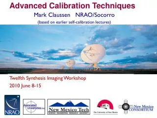
Advanced Calibration Techniques Crystal Brogan (NRAO / North American ALMA Science Center)
Outline • The Troposphere • Mean effect • Correcting for atmospheric noise and attenuation • Phase Fluctuations / Decorrelation • Phase Correction Techniques • Techniques • Self-calibration • WVRs • Absolute Flux Calibration
Column Density as a Function of Altitude Constituents of Atmospheric Opacity Due to the troposphere (lowest layer of atmosphere): h < 10 km Temperature with altitude: clouds & convection can be significant Dry Constituents of the troposphere:, O2, O3, CO2, Ne, He, Ar, Kr, CH4, N2, H2 H2O: abundance is highly variable but is < 1% in mass, mostly in the form of water vapor “Hydrosols” (water droplets in clouds and fog) also add a considerable contribution when present Stratosphere Troposphere
At 1.3cm most opacity comes from H2O vapor • At 7mm biggest contribution from dry constituents • At 3mm both components are significant • “hydrosols” i.e. water droplets (not shown) can also add significantly to the opacity total optical depth Opacity optical depth due to H2O vapor Optical Depth as a Function of Frequency optical depth due to dry air 43 GHz 7mm Q band 100 GHz 3mm MUSTANG 22 GHz 1.3cm K band ALMA
Atmospheric Opacity at ALMA (PWV = Precipitable Water Vapor) O3 O2 H2O H2O H2O H2O
TroposphericOpacity Depends on Altitude: Altitude: 5000 m ALMA PWV= 1mm O2H2O Altitude: 2150 m Models of atmospheric transmission from 0 to 1000 GHz for the ALMA site in Chile, and for the VLA site in New Mexico The difference is due primarily to the scale height of water vapor, not the “dryness” of the site. Þ Atmosphere transmission not a problem for l > cm (most VLA bands) EVLA PWV= 4mm PWV = depth of H2O if converted to liquid
This refraction causes: • - Pointing off-sets, Δθ≈ 2.5x10⁻⁴xtan(i) (radians) • @ elevation 45o typical offset~1’ • - Delay (time of arrival) off-sets • These “mean” errors are generally removed by the online system Mean Effect of Atmosphere on Phase • Since the refractive index of the atmosphere ≠1, an electromagnetic wave propagating through it will experience a phase change (i.e. Snell’s law) • The phase change is related to the refractive index of the air, n, and the distance traveled, D, by • fe = (2p/l) ´n´D • For water vapor nµw • DTatm • so fe»12.6p´wfor Tatm = 270 K • l w=precipitable water vapor (PWV) column Tatm = Temperature of atmosphere
so Tnoise≈Trx+Tatm(1-e-t) Receiver temperature Emission from atmosphere • Consider the signal-to-noise ratio: • S / N = (Tsourcee-t) / Tnoise= Tsource / (Tnoiseet) • Tsys= Tnoiseet ≈Tatm(et-1) + Trxet Tnoise≈Trx+ Tsky where Tsky =Tatm (1 – e-t) + Tbge-t Tatm = temperature of the atmosphere ≈ 300 K Tbg = 3 K cosmic background For a perfect antenna, ignoring spillover and efficiencies Sensitivity: System noise temperature Before entering atmosphere the source signal S= Tsource After attenuation by atmosphere the signal becomes S=Tsourcee- In addition to receiver noise, at millimeter wavelengths the atmosphere has a significant brightness temperature (Tsky): • The system sensitivity drops rapidly (exponentially) as opacity increases
Impact of Atmospheric Noise Assuming Tatm = 300 K, elevation=40 degrees, ignoring antenna efficiencies • Tsys≈Tatm(et-1) + Trxet • JVLA Qband (43 GHz) • typical winter PWV = 5 mm τzenith=0.074 τ40= 0.115 • typical Trx=35 K • Tsys = 76 K • ALMA Band 6 (230 GHz) • typical PWV = 1.8 mm τzenith=0.096 τ40= 0.149 • typical Trx=50 K • Tsys= 106 K • ALMA Band 9 (690 GHz) • typical PWV = 0.7 mm τzenith=0.87 τ40= 1.35 • typical Trx= 150 K • Tsys= 1435 K
Vin =G Tin = G [Trx+ Tload] Vout= G Tout = G [Trx+Tatm(1-e-t) +Tbge-t +Tsourcee-t] Load in Load out assume Tatm≈ Tload Vin – VoutTload VoutTsys Comparing in and out = Tsys = Tload * Tout / (Tin – Tout) SMA calibration load swings in and out of beam Power is really observed but is T in the R-J limit • The “chopper wheel” method: putting an ambient temperature load (Tload) in front of the receiver and measuring the resulting power compared to power when observing sky Tatm (Penzias & Burrus 1973). Measurement of Tsysin the Sub(millimeter) How do we measureTsys = Tatm(et-1) + Trxetwithout constantly measuring Trx and the opacity? • IF Tatm≈Tload, and Tsys is measured often, changes in mean atmospheric absorption are corrected. ALMA has a two temperature load system which allows independent measure of Trx
ALMA System Temperature: Example-1 Elevation vs. Time ALMA Band 9 Test Data on the quasar NRAO530 • Notice: • Inverse relationship between elevation and Tsys • Large variation of Tsys among the antennas Tsys vs. Time (all antennas)
ALMA System Temperature: Example-2 Tsys vs. Time (all antennas) Raw Amplitude vs. Time Fully Calibrated using flux reference Amplitude Corrected for Tsys Sfinal ~ STsys* Antenna Efficiency Factor (about 40 Jy/K for ALMA)
JVLA Switched Power • Alternative to a mechanical load system is a switched “calibration diode” • Broad band, stable noise (Tcal~3K) is injected into receiver at ~20 Hz • Synchronous detector downstream of gives sum & difference powers • Advantages • Removes all gain variations due to the analog electronics between A and B • Puts data on absolute temperature scale • Caveats: • Does not account for opacity effects • Does not account for antenna gain curve
JVLA Switched Power Example Antenna Gain as a function of time This is what you get if you apply switched power first, large variations with time are removed Gain solutions from calibrator-based calibration; all the sources are strong calibrators A science source will have similar (large) gain variations with time, and only if you switch frequently to a strong calibrator for gain solutions can you TRY to take out these variations. This calibration takes out electronic but not ionospheric or tropospheric gain variations. The latter would still need to be taken out by calibrator (or other calibration) observations.
JVLA Atmospheric Correction • At higher frequencies still need to account for atmospheric opacity and antenna gain variations with elevation (i.e. antenna gain curves) plotweather task available in CASA3.4 Hopefully in the future a “tipper” that directly monitors the atmospheric opacity will provide more accurate estimates Optical depth at zenith
Atmospheric phase fluctuations You can observe in apparently excellent submm weather (in terms of transparency) and still have terrible “seeing” i.e. phase stability. Variations in the amount of precipitable water vapor (PWV) cause phase fluctuations, which are worse at shorter wavelengths (higher frequencies), and result in: Low coherence (loss of sensitivity) Radio “seeing”, typically 0.1-1² at 1 mm Anomalous pointing offsets Anomalous delay offsets Patches of air with different water vapor content (and hence index of refraction) affect the incoming wave front differently.
“Root phase structure function” (Butler & Desai 1999) • RMS phase fluctuations grow as a function of increasing baseline length until break when baseline length ≈ thickness of turbulent layer • The position of the break and the maximum noise are weather and wavelength dependent Atmospheric phase fluctuations, continued… log (RMS Phase Variations) Break Phase noise as function of baseline length Log (Baseline Length) • RMS phase of fluctuations given by Kolmogorov turbulence theory • frms = K ba / l [deg] • b= baseline length (km) • = 1/3 to 5/6 (thin atmosphere vs. thick atmosphere) • = wavelength (mm) K = constant (~100 for ALMA, 300 for JVLA)
Residual Phase and Decorrelation Q-band (7mm) VLA C-config. data from “good” day An average phase has been removed from absolute flux calibrator 3C286 Coherence = (vector average/true visibility amplitude) = áVñ/ V0 Where, V = V0eif The effect of phase noise, frms, on the measured visibility amplitude : áVñ = V0´áeifñ = V0´e-f2rms/2(Gaussian phase fluctuations) Example: if frms = 1 radian (~60 deg), coherence = áVñ = 0.60V0 Short baseline Long baseline For these data, the residual rms phase (5-20 degrees) from applying an average phase solution produces a 7% error in the flux scale (minutes) • Residual phase on long baselines have larger excursions, than short baselines
Corrections 30min: Corrections 30sec: All data: Reduction in peak flux (decorrelation) and smearing due to phase fluctuations over 60 min No sign of phase fluctuations with timescale ~ 30 s one-minute snapshots at t = 0 and t = 59 minutes Sidelobe pattern shows signature of antenna based phase errors small scale variations that are uncorrelated Position offsets due to large scale structures that are correlatedphase gradient across array 22 GHz VLA observations of the calibrator 2007+404 resolution of 0.1” (Max baseline 30 km) • Uncorrelated phase variations degrades and decorrelates image Correlated phase offsets = position shift
Phase fluctuation correction methods Fast switching: An Observing strategy - used at the EVLA for high frequencies and will be used at ALMA. Choose fast switching cycle time, tcyc, short enough to reduceΦrmsto an acceptable level. Calibrate in the normal way. Self-calibration:Goodfor bright sources that can be detected in a few seconds. Radiometer: Monitor phase (via path length) with special dedicated receivers Phase transfer:simultaneously observe low and high frequencies, and transfer scaled phase solutions from low to high frequency. Can be tricky, requires well characterized system due to differing electronics at the frequencies of interest. Paired array calibration: divide array into two separate arrays, one for observing the source, and another for observing a nearby calibrator. Will not remove fluctuations caused by electronic phase noise Can only work for arrays with large numbers of antennas (e.g., CARMA, JVLA, ALMA)
Self-Calibration: Motivation JVLA and ALMA have impressive sensitivity! Many objects will have enough Signal-to-Noise (S/N) so they can be used to better calibrate themselves to obtain a more accurate image. This is called self-calibration and it really works, if you are careful! Sometimes, the increase in effective sensitivity may be an order of magnitude. It is not a circular trick to produce the image that you want. It works because the number of baselines is much larger than the number of antennas so that an approximate source image does not stop you from determining a better temporal gain calibration which leads to a better source image. Self-cal may not be included in the data pipelines. SO, YOU SHOULD LEARN HOW TO DO IT.
Data Corruption Types • The true visibility is corrupted by many effects: • Atmospheric attenuation • Radio “seeing” • Variable pointing offsets • Variable delay offsets • Electronic gain changes • Electronic delay changes • Electronic phase changes • Radiometer noise • Correlator mal-functions • Most Interference signals | Antenna-based | baseline
Antenna-based Calibration- I • The most important corruptions are associated with antennas • Basic Calibration Equation Factorable (antenna-based) complex gains Non-factorable complex gains (not Antenna based) True Visibility Additive offset (not antenna based) and thermal noise, respectively • Can typically be reduced to approximately
Antenna-based Calibration-II • For N antennas, [(N-1)*N]/2 visibilities are measured, but only N amplitude and (N-1) phase gains fully describe the complete calibration. This redundancy is used for antenna gain calibration • Basic gain (phase and amplitude) calibration involves observing unresolved (point like) “calibrators” of known position with visibility Mi,j (tk, n) • Determine gain corrections, gi, that minimizes Sk for each time stamp tkwhere • The solution interval, tk, is the data averaging time used to obtain the values of gi, typically [solint=‘int’ or ‘inf’] The apriori weight of each data point is wi,j. • This IS a form of Self-calibration, only we assumea Model (Mij) that has constant amplitude and zero phase, i.e. a point source • The transfer of these solutions to another position on the sky at a different time (i.e. your science target) will be imperfect, but the same redundancy can be used with a model image for Self-calibration
Self-Calibration Equation • The clean model from making an image can be compared to the data, and differential gains can be found that minimize the differences Complex Visibilities Fourier transform of model image Data Weights Complex Gains • is the corrected visibility data after normal gain calibration Are the new complex gain corrections you are looking for
Sensitivities for Self-Calibration-I • For phase only self-cal: Need to detect the target in a solution time (solint) < the time for significant phase variations with only the baselines to a single antenna with a S/Nself > 3. For 25 antennas, S/NSelf > 3 will lead to < 15 deg error. • Make an initial image, cleaning it conservatively • Measure rms in emission free region • rmsAnt = rmsx sqrt(N-3) where N is # of antennas • rmsself = rmsAntxsqrt(total time/solint) • Measure peak flux density = Signal • If S/Nself = Peak/rmsSelf>3 try phase only self-cal Rule of thumb: If S/N in image >20 you can usually self-cal • CAVEAT: If dominated by extended emission, estimate what the flux will be on the longer baselines (by plotting the uv-data) instead of the image • If the majority of the baselines in the array cannot "see" the majority of emission in the target field (i.e. emission is resolved out) at a S/N of about 3, the self-cal will fail in extreme cases (though bootstrapping from short to longer baselines is possible it can be tricky). • CAVEAT: If severely dynamic range limited (poor uv-coverage), it can also be helpful to estimate the rms noise from uv-plots
Sensitivities for Self-Calibration-II • For amplitude self-cal: Need to detect the target with only the baselines to a single antenna with a S/N > 10, in a solution time (solint) < the time for significant amplitude variations. For 25 antennas, an antenna based S/N > 10 will lead to a 10% amplitude error. • If clean model is missing significant flux compared to uv-data, give uvrange for amplitude solution that excludes short baselines Additional S/N can be obtained by: • Increase solint (solution interval) • gaintype= ‘T’ to average polarizations • Caveat 1: Only if your source is unpolarized • Combine = ‘spw’ to average spw’s • Caveat 1: if your observing frequency / bandwidth ratio is < 10 so that changes in source morphology are seen across the band, do not combine spws for any self-cal • Caveat 2: if your source spectral index changes significantly across the band, do not combine spws for amplitude self-cal • Combine = ‘fields’ to average fields in a mosaic (use with caution)
Self-calibration Example: ALMA SV Data for IRAS16293 Band 6 (Ia) • Step 1 – Determine basic setup of data: • 2 pointing mosaic • Integration = 6.048 sec; subscans ~ 30sec • Scan= 11min 30s (split between two fields) • Step 2 – What is the expected rms noise? • Use actual final total time and # of antennas on science target(s) from this stage and sensitivity calculator. • Be sure to include the actual average weather conditions for the observations in question and the bandwidth you plan to make the image from • 54 min per field with 16 antennas and average Tsys ~ 80 K, 9.67 MHz BW; rms= 1 mJy/beam • Inner part of mosaic will be about 1.6 x better • ALMA mosaic: alternates fields in “subscan” this picture = 1 scan • EVLA mosaic: alternates fields in scans • Subscans are transparent to CASA (and AIPS)
Self-calibration Example: ALMA SV Data for IRAS16293 Band 6 (Ib) • Step 3 – What does the amplitude vsuv-distance of your source look like? • Does it have large scale structure? i.e. increasing flux on short baselines. • What is the flux density on short baselines? • Keep this 4 Jy peak in mind while cleaning. What is the total cleaned flux you are achieving?
Self-calibration Example: ALMA SV Data for IRAS16293 Band 6 (II) • Step 3 – What is the S/N in a conservatively cleaned image? • What is this “conservative” of which you speak • Rms~ 15 mJy/beam; Peak ~ 1 Jy/beam S/N ~ 67 • Rms > expected and S/N > 20 self-cal! Stop clean, and get rms and peak from image, avoiding negative bowls and emission Clean boxes only around emission you are SURE are real at this stage Residual after 200 iterations
Self-calibration Example: ALMA SV Data for IRAS16293 Band 6 (III) • Step 4: Decide on an time interval for initial phase-only self-cal • A good choice is often the scan length (in this case about 5 minutes per field) • Exercise for reader: from page 27 show that S/Nself ~ 5.4 • In CASA you can just set solint=‘inf’ (i.e. infinity) and as long as combine ≠ ‘scan’ AND ≠ ‘field’ you will get one solution per scan, per field. • Use ‘T’ solution to combine polarizations • What to look for: • Lot of failed solutions on most antennas? if so, go back and try to increase S/N of solution = more averaging of some kind • Do the phases appear smoothly varying with time (as opposed to noise like)
Self-calibration Example: ALMA SV Data for IRAS16293 Band 6 (IV) • Step 5: Apply solutions and re-clean • Incorporate more emission into clean box if it looks real • Stop when residuals become noise-like but still be a bit conservative, ESPESCIALLY for weak features that you are very interested in • You cannot get rid of real emission by not boxing it • You can create features by boxing noise Original • Step 6: Compare Original clean image with 1st phase-only self-cal image • Original: • Rms~ 15 mJy/beam; Peak ~ 1 Jy/beam S/N ~ 67 • 1st phase-only: • Rms~ 6 mJy/beam; Peak ~ 1.25 Jy/beam S/N ~ 208 • Did it improve? If, yes, continue. If no, something has gone wrong or you need a shorter solint to make a difference, go back to Step 4 or stop. 1st phase cal
Self-calibration Example: ALMA SV Data for IRAS16293 Band 6 (V) • Step 5:Try shorter solint for 2nd phase-only self-cal • In this case we’ll try the subscan length of 30sec • It is best NOT to apply the 1st self-cal while solving for the 2nd. i.e. incremental tables can be easier to interpret but you can also “build in” errors in first model by doing this • What to look for: • Still smoothly varying? • If this looks noisy, go back and stick with longer solint solution • IF this improves things a lot, could try going to even shorter solint
Self-calibration Example: ALMA SV Data for IRAS16293 Band 6 (VI) • Step 6: Apply solutions and re-clean • Incorporate more emission into clean box if it looks real • Stop when residuals become noise-like but still be a bit conservative, ESPECIALLY for weak features that you are very interested in • You cannot get rid of real emission by not boxing it • You can create features by boxing noise 1st phase cal • Step 7: Compare 1st and 2nd phase-only self-cal images • 1st phase-only: • Rms~ 6 mJy/beam; Peak ~ 1.25 Jy/beam S/N ~ 208 • 2nd phase-only: • Rms~ 5.6 mJy/beam; Peak ~ 1.30 Jy/beam S/N ~ 228 • Did it improve? Not much, so going to shorter solint probably won’t either, so we’ll try an amplitude self-cal next 2nd phase cal
Self-calibration Example: ALMA SV Data for IRAS16293 Band 6 (VII) Residual phase • Step 8:Try amplitude self-cal • Amplitude tends to vary more slowly than phase. It’s also less constrained, so solints are typically longer. Lets try two scans worth or 23 minutes • Essential to apply the best phase only self-cal before solving for amplitude. Also a good idea to use mode=‘ap’ rather than just ‘a’ to check that residual phase solutions are close to zero. • Again make sure mostly good solutions, and a smoothly varying pattern. Scale +/- 10 degrees Amplitude Scale 0.8 to 1.0
Self-calibration Example: ALMA SV Data for IRAS16293 Band 6 (VIII) • Step9: Apply solutions • Apply both 2nd phase and amp cal tables • Inspect uv-plot of corrected data to • Check for any new outliers, if so flag and go back to Step 9. • Make sure model is good match to data. • Confirm that flux hasn’t decreased significantly after applying solutions Original Amp & Phase applied Image Model (total cleaned flux = 3.4 Jy)
Self-calibration Example: ALMA SV Data for IRAS16293 Band 6 (IX) • Step 10: Re-clean • Incorporate more emission into clean box • Stop when residuals become noise-like – clean everything you think is real Original • Step 11: Compare 2nd phase-only and amp+phase self-cal images • 2nd phase-only: • Rms~ 5.6 mJy/beam; Peak ~ 1.30 Jy/beam S/N ~ 228 • Amp & Phase: • Rms~4.6 mJy/beam; Peak~1.30 Jy/beam S/N ~283 • Did it improve? Done! 2nd phase cal Final: S/N=67 vs 283! But not as good as theoretical = dynamic range limit Amp & Phase cal
Self-Calibration example 2: JVLAWater Masers (I) uv-spectrum after standard calibrator-based calibration for bandpass and antenna gains There are 16 spectral windows, 8 each in two basebands (colors in the plot) Some colors overlap because the basebands were offset in frequency by ½ the width of an spw in order to get good sensitivity across whole range. The continuum of this source is weak. How do you self-cal this? • Make an image • If you want to speed things up, limit the velocity to the region with strong emission in the uv-plot: -20 to 0 km/s in this case. • Then look at the model data column the same way
Self-Calibration example 2: JVLAWater Masers (II) Model from initial clean image, zoomed in to the velocity range imaged: -20 to 0 km/s. But to calibrate we need to know the SPWs and the CHANNELs with strong emission in the model: CASA’splotms with locate can help
Self-Calibration example 2: JVLAWater Masers (IV) Model from initial clean image, zoomed in to the velocity range imaged: -20 to 0 km/s. But to calibrate we need to know the SPWs and the CHANNELs with strong emission in the model: CASA’splotms with locate can help • From the locate we find a strong set of channels in • spw=3 channels 12~22 • spw=12 channels 76~86 • We use these channels in the self-calibration. • It is very important not to include channels with no signal in the clean model!
Self-Calibration example 2: JVLAWater Masers (V) Final self-calibrated spectrum • One remaining trickiness: calibration solutions are only for spw=3 and 12. The spwmap parameter can be used to map calibration from one spectral window to another. There must be an entry for all spws: • spwmap=[3,3,3,3,3,3,3,3,12,12,12,12,12,12,12,12] • In other words apply the spw=3 calibration to the 8 spectral windows in the lower baseband and the calibration from spw=12 to the 8 spws in the upper baseband • Beyond this everything is the same as previous example.
183 GHz Radiometers: w=precipitable water vapor (PWV) column 22 GHz Radiometry: measure fluctuations in TBatm with a radiometer, use these to derive changes in water vapor column (w) and convert this into a phase correction using fe»12.6p´w l (Bremer et al. 1997) Monitor: 22 GHz H2O line (CARMA, VLA) 183 GHz H2O line (CSO-JCMT, SMA, ALMA) total power (IRAM)
ALMA WVR System There are 4 “channels” flanking the peak of the 183 GHz water line Installed on all the 12m antennas • Data taken every second • Matching data from opposite sides are averaged • The four channels allow flexibility for avoiding saturation • Next challenges are to perfect models for relating the WVR data to the correction for the data • An atmospheric model is used for the dry component • It works pretty well already!
ALMA WVR Correction - Examples Band 7 (340 GHz) Extended config Band 6 (230 GHz) Compact config Raw phase &WVR corrected phase
Flux calibrators – JVLA JVLA Flux Calibrators 3C 48 (0137+331) 3C286 (1331+305) 3C138 (0521+166) 3C147 (0542+498) Stable brightness and morphology, but are resolved on long baselines and high frequencies. An image model must be used
Flux calibrators – ALMA • Quasars are strongly time-variable and good models do not exist at higher frequencies • Solar system bodies are used as primary flux calibrators (Neptune, Jovian moons, Titan, Ceres) but with many challenges: • All are resolved on long ALMA baselines • Brightness varies with distance from Sun and Earth • Line emission (Neptune, Titan) • More asteroids? modeling is needed because they are not round! • Red giant stars may be better • Regular monitoring of a small grid of point-like quasars as secondary flux calibrators. Ceres 690 GHz ALMA extended Neptune, 690 GHz ALMA compact config UV distance UV distance