Download
1 / 49
520 likes | 965 Views
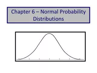
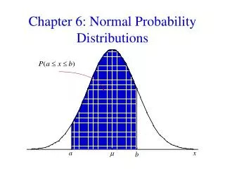
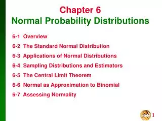
Overview The Standard Normal Distribution Normal Distributions: Finding Probabilities Normal Distributions: Finding Values The Central Limit Theorem. Chapter 6 Normal Probability Distributions. Continuous random variable Normal distribution. Curve is bell shaped and symmetric. µ

E N D
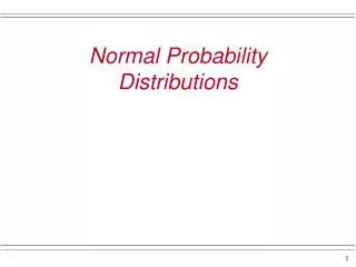
Overview The Standard Normal Distribution Normal Distributions: Finding Probabilities Normal Distributions: Finding Values The Central Limit Theorem Chapter 6Normal Probability Distributions
Continuous random variable Normal distribution Curve is bell shaped and symmetric µ Score Overview x - µ2 ( ) 1 2 y = e 2 p
Density Curve (or probability density function) the graph of a continuous probability distribution Definitions 1. The total area under the curve must equal 1. 2. Every point on the curve must have a vertical height that is 0 or greater.
Because the total area under the density curve is equal to 1, there is a correspondence between area and probability.
Women: µ = 63.6 = 2.5 Heights of Adult Men and Women Men: µ = 69.0 = 2.8 63.6 69.0 Height (inches)
Standard Normal Deviation a normal probability distribution that has a mean of 0 and a standard deviation of 1 Definition
The Empirical Rule Standard Normal Distribution: µ = 0 and = 1 0.1% 99.7% of data are within 3 standard deviations of the mean 95% within 2 standard deviations 68% within 1 standard deviation 34% 34% 2.4% 2.4% 0.1% 13.5% 13.5% x - 3s x - 2s x - s x x+s x+2s x+3s
P(a < z < b) denotes the probability that the z score is between a and b P(z > a) denotes the probability that the z score is greater than a P (z < a) denotes the probability that the z score is less than a Notation
Finding the Area to the Right of z= 1.27 This area is 0.1020 z = 1.27 0
the distance along horizontal scale of the standard normal distribution; refer to the leftmost column and top rowof theTable Area the region under the curve; refer to the values in the body of the Table To find:zScore
µ = 0 = 1 Table E Standard Normal Distribution 0 x z
Standard Normal Deviation a normal probability distribution that has a mean of 0 and a standard deviation of 1 -3 -2 -1 0 1 2 3 Definition Area found in Table A2 Area = 0.3413 0.4429 z = 1.58 0 Score (z )
Example: If thermometers have an average (mean) reading of 0 degrees and a standard deviation of 1 degree for freezing water and if one thermometer is randomly selected, find the probability that it reads freezing water between 0 degrees and 1.58 degrees.
The probability that the chosen thermometer will measure freezing water between 0 and 1.58 degrees is 0.4429. Example: If thermometers have an average (mean) reading of 0 degrees and a standard deviation of 1 degree for freezing water and if one thermometer is randomly selected, find the probability that it reads freezing water between 0 degrees and 1.58 degrees. Area = 0.4429 P ( 0 < x < 1.58 ) = 0.4429 0 1.58
The probability that the chosen thermometer will measure freezing water between -2.43 and 0 degrees is 0.4925. Example: If thermometers have an average (mean) reading of 0 degrees and a standard deviation of 1 degree for freezing water, and if one thermometer is randomly selected, find the probability that it reads freezing water between -2.43 degrees and 0degrees. Area = 0.4925 P ( -2.43 < x < 0 ) = 0.4925 -2.43 0
Finding the Area Between z= 1.20 and z = 2.30 Area A is 0.1044 A z= 1.20 z= 2.30 0
x - µ z = Other Normal Distributions If 0or 1 (or both), we will convert values to standard scores using Formula 5-2, then procedures for working with all normal distributions are the same as those for the standard normal distribution.
x - z = Converting to Standard Normal Distribution P P x z 0 (a) (b)
Probability of Weight between 143 pounds and 201 pounds 201 - 143 z = = 2.00 29 x = 143 s=29 Weight 143201 z 0 2.00
Probability of Weight between 143 pounds and 201 pounds OR - 47.72% of women have weights between 143 lb and 201 lb. x = 143 s=29 Weight 143201 z 0 2.00
2nd Distributions 2:normalcdf (lower bound, upper bound, mean, s.d.) Finding a probability when given a z-score using the TI83
1. Draw a bell-shaped curve, draw the centerline, and identify the region under the curve that corresponds to the given probability. If that region is not bounded by the centerline, work with a known region that is bounded by the centerline. 2. Using the probability representing the area bounded by the centerline, locate the closest probability in the body of Table E and identify the corresponding z score. 3. If the z score is positioned to the left of the centerline, make it a negative. Finding a z - score when given a probabilityUsing the Table
Finding z Scores when Given Probabilities 95% 5% 5% or 0.05 0.45 0.50 1.645 0 (z score will be positive) Finding the 95th Percentile
Finding z Scores when Given Probabilities 90% 10% Bottom 10% 0.10 0.40 -1.28 0 (zscore will be negative) Finding the 10th Percentile
2nd Distributions 3:Invnorm (%,mean,s.d) Finding z Scores when Given ProbabilitiesUsing the TI83
1. Don’t confuse zscores and areas. Z scores are distances along the horizontal scale, but areas are regions under the normal curve. Table A-2 lists z scores in the left column and across the top row, but areas are found in the body of the table. 2. Choose the correct (right/left) side of the graph. 3. A z score must be negative whenever it is located to the left of the centerline of 0. Cautions to keep in mind
Finding z Scores when Given Probabilities 95% 5% 5% or 0.05 0.45 0.50 1.645 0 (z score will be positive) Finding the 95th Percentile
Finding z Scores when Given Probabilities 90% 10% Bottom 10% 0.10 0.40 -1.28 0 (zscore will be negative) Finding the 10th Percentile
1. Sketch a normal distribution curve, enter the given probability or percentage in the appropriate region of the graph, and identify thexvalue(s) being sought. Use Table E to find the z score corresponding to the region bounded by x and the centerline of 0. Cautions: Refer to the BODY of Table E to find the closest area, then identify the corresponding zscore. Make thez score negative if it is located to the left of the centerline. 3. Using the Formula, enter the values for µ, , and thez score found in step 2, then solve forx. x= µ + (z• ) 4. Refer to the sketch of the curve to verify that the solution makes sense in the context of the graph and the context of the problem. Procedure for Finding Values Using the Table and By Formula
Finding P10 for Weights of Women 10% 90% 40% 50% Weight x = ? 143
Finding P10 for Weights of Women The weight of 106 lb (rounded) separates the lowest 10% from the highest 90%. 0.10 0.40 0.50 Weight x = 106 143 0 -1.28
Forgot to make z score negative??? UNREASONABLE ANSWER! 0.10 0.40 0.50 Weight x = 180 143 0 1.28
REMEMBER! Make the z score negative if the value is located to the left (below) the mean. Otherwise, the z score will be positive.
Definition Sampling Distribution of the mean the probability distribution of sample means, with all samples having the same sample size n.
1. The random variable xhas a distribution (which may or may not be normal) with mean µ and standard deviation . 2. Samples all of the same size n are randomly selected from the population of xvalues. Central Limit Theorem Given:
Central Limit Theorem Conclusions: 1. The distribution of sample x will, as the sample size increases, approach a normal distribution. 2. The mean of the sample means will be the population mean µ. 3. The standard deviation of the sample means will approach n
1. For samples of size n larger than 30, the distribution of the sample means can be approximated reasonably well by a normal distribution. The approximation gets better as the sample size n becomes larger. 2. If the original population is itself normally distributed, then the sample means will be normally distributed for any sample sizen (not just the values of n larger than 30). Practical Rules Commonly Used:
the mean of the sample means the standard deviation of sample mean (often called standard error of the mean) Notation µx= µ x= n
0 Distribution of 200 digits from Social Security Numbers (Last 4 digits from 50 students) 20 Frequency 10 0 1 2 3 4 5 6 7 8 9 Distribution of 200 digits
1 5 9 5 9 4 7 9 5 7 8 3 8 1 3 2 7 1 3 6 3 8 2 3 6 1 5 3 4 6 4 6 8 5 5 2 6 4 9 4.75 4.25 8.25 3.25 5.00 3.50 5.25 4.75 5.00 2 6 2 2 5 0 2 7 8 5 3 7 7 3 4 4 4 5 1 3 6 7 3 7 3 3 8 3 7 6 2 6 1 9 5 7 8 6 4 0 7 4.00 5.25 4.25 4.50 4.75 3.75 5.25 3.75 4.50 6.00 SSN digits x
0 Distribution of 50 Sample Means for 50 Students 15 Frequency 10 5 0 1 2 3 4 5 6 7 8 9
As the sample size increases, the sampling distribution of sample means approaches a normal distribution.
Example: Given the population of women has normally distributed weights with a mean of 143 lb and a standard deviation of 29 lb, a.) if one woman is randomly selected, find the probability that her weight is greater than 150 lb.b.) if 36 different women are randomly selected, find the probability that their mean weight is greater than 150 lb.
Example: Given the population of women has normally distributed weights with a mean of 143 lb and a standard deviation of 29 lb, a.) if one woman is randomly selected, the probability that her weight is greater than 150 lb. is 0.4052. 0.5 - 0.0948 = 0.4052 0.0948 = 143 150 = 29 0 0.24
Example: Given the population of women has normally distributed weights with a mean of 143 lb and a standard deviation of 29 lb, b.) if 36 different women are randomly selected, the probability that their mean weight is greater than 150 lb is 0.0735. z = 150-143 = 1.45 29 36 0.5 - 0.4265 = 0.0735 0.4265 x = 143 150 x= 4.83333 0 1.45
a.) if one woman is randomly selected, find the probability that her weight is greater than 150 lb.P(x > 150) = 0.4052 b.) if 36 different women are randomly selected, their mean weight is greater than 150 lb.P(x > 150) = 0.0735It is much easier for an individual to deviate from the mean than it is for a group of 36 to deviate from the mean. Example: Given the population of women has normally distributed weights with a mean of 143 lb and a standard deviation of 29 lb,
2nd Distributions 2:normalcdf (lower bound, upper bound, mean, s.e) Replace s.d. with standard error Finding a z - score for a group Using TI83