Download
1 / 27

E N D
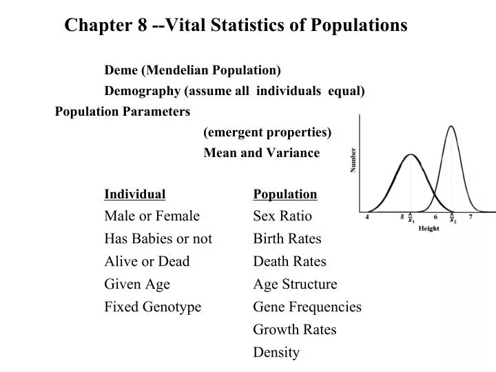
Chapter 8 --Vital Statistics of Populations Deme (Mendelian Population) Demography (assume all individuals equal) Population Parameters (emergent properties) Mean and VarianceIndividualPopulation Male or Female Sex Ratio Has Babies or not Birth Rates Alive or Dead Death Rates Given Age Age Structure Fixed Genotype Gene Frequencies Growth Rates Density
Life tables: Horizontal versus vertical samples Segment Cohort Age Birth Time
Life TablesDiscrete versus Continuous Ages Pivotal Age assumption (age classes)qx = force of mortality (fraction dying during age interval)qx = age-specific death rate Survivorship curveslx = fraction of initial cohort that survives to age xly / lx = probability of living from age x to age yEx = Expectation of further life
Type 1: Rectangular Type 2: Diagonal Type 3: Inverse Hyperbolic Xantusia vigilis sheep Uta stansburiana
Xantusia vigilis Eumeces fasciatus Eumeces fasciatus Sceloporus olivaceus
Fecundity, Tables of Reproductionmx = age-specific fecundity Two conventions: females only, or count both males and females but weight each as one-half (only progeny entering age class zero are counted) Gross reproductive rate (GRR) is the sum of mx over all ages However, because some females will die before having all their possible babies, must calculate realized fecundity which is simply lxmx (the fraction of females surviving times their fecundity) Realized fecundity, lxmx, is summed over all ages to get the Net Reproductive Rate, R0 (also called the Replacement Rate of the Population)
http://www.zo.utexas.edu/courses/THOC/breeders.html http://www.oregonlive.com/kiddo/index.ssf/2008/05/environmental_moms_stop_at_one.html
http://en.wikipedia.org/wiki/Quiverfull http://www.oregonlive.com/kiddo/index.ssf/2008/05/environmental_moms_stop_at_one.html
http://www.zo.utexas.edu/courses/THOC/breeders.html http://www.oregonlive.com/kiddo/index.ssf/2008/05/environmental_moms_stop_at_one.html
0 1 2 3 4 5 mm Pediculus humanus Human Body Louse
T, Generation time = average time from one gener- ation to the next (average time from egg to egg) vx= Reproductive Value = Age-specific expectation of all future offspring p.143, right hand equation “dx” should be “dt”
vx = mx + (lt / lx ) mt Residual reproductive value = age-specific expectation of offspring in distant futurevx* = ( lx+1 / lx ) vx+1
Illustration of Calculation of Ex, T, R0, and vx in a Stable Population with Discrete Age Classes _____________________________________________________________________ Age Expectation Reproductive Weighted of Life Value Survivor- Realized by Realized Ex vx Age (x) ship Fecundity Fecundity Fecundity lx mx lxmx x lxmx _____________________________________________________________________ 0 1.0 0.0 0.00 0.00 3.40 1.00 1 0.8 0.2 0.16 0.16 3.00 1.25 2 0.6 0.3 0.18 0.36 2.67 1.40 3 0.4 1.0 0.40 1.20 2.50 1.65 4 0.4 0.6 0.24 0.96 1.50 0.65 5 0.2 0.1 0.02 0.10 1.00 0.10 6 0.0 0.0 0.00 0.00 0.00 0.00 Sums 2.2 (GRR) 1.00 (R0) 2.78 (T) _____________________________________________________________________ E0 = (l0 + l1 + l2 + l3 + l4 + l5)/l0 = (1.0 + 0.8 + 0.6 + 0.4 + 0.4 + 0.2) / 1.0 = 3.4 / 1.0 E1 = (l1 + l2 + l3 + l4 + l5)/l1 = (0.8 + 0.6 + 0.4 + 0.4 + 0.2) / 0.8 = 2.4 / 0.8 = 3.0 E2 = (l2 + l3 + l4 + l5)/l2 = (0.6 + 0.4 + 0.4 + 0.2) / 0.6 = 1.6 / 0.6 = 2.67 E3 = (l3 + l4 + l5)/l3 = (0.4 + 0.4 + 0.2) /0.4 = 1.0 / 0.4 = 2.5 E4 = (l4 + l5)/l4 = (0.4 + 0.2) /0.4 = 0.6 / 0.4 = 1.5 E5 = (l5) /l5 = 0.2 /0.2 = 1.0 v1 = (l1/l1)m1+(l2/l1)m2+(l3/l1)m3+(l4/l1)m4+(l5/l1)m5 = 0.2+0.225+0.50+0.3+0.025 = 1.25 v2 = (l2/l2)m2 + (l3/l2)m3 + (l4/l2)m4 + (l5/l2)m5 = 0.30+0.67+0.40+ 0.03 = 1.40 v3 = (l3/l3)m3 + (l4/l3)m4 + (l5/l3)m5 = 1.0 + 0.6 + 0.05 = 1.65 v4 = (l4/l4)m4 + (l5/l4)m5 = 0.60 + 0.05 = 0.65 v5 = (l5/l5)m5 = 0.1 ___________________________________________________________________________
Illustration of Calculation of Ex, T, R0, and vx in a Stable Population with Discrete Age Classes _____________________________________________________________________ Age Expectation Reproductive Weighted of Life Value Survivor- Realized by Realized Ex vx Age (x) ship Fecundity Fecundity Fecundity lx mx lxmx x lxmx _____________________________________________________________________ 0 1.0 0.0 0.00 0.00 3.40 1.00 1 0.8 0.2 0.16 0.16 3.00 1.25 2 0.6 0.3 0.18 0.36 2.67 1.40 3 0.4 1.0 0.40 1.20 2.50 1.65 4 0.4 0.6 0.24 0.96 1.50 0.65 5 0.2 0.1 0.02 0.10 1.00 0.10 6 0.0 0.0 0.00 0.00 0.00 0.00 Sums 2.2 (GRR) 1.00 (R0) 2.78 (T) _____________________________________________________________________ E0 = (l0 + l1 + l2 + l3 + l4 + l5)/l0 = (1.0 + 0.8 + 0.6 + 0.4 + 0.4 + 0.2) / 1.0 = 3.4 / 1.0 E1 = (l1 + l2 + l3 + l4 + l5)/l1 = (0.8 + 0.6 + 0.4 + 0.4 + 0.2) / 0.8 = 2.4 / 0.8 = 3.0 E2 = (l2 + l3 + l4 + l5)/l2 = (0.6 + 0.4 + 0.4 + 0.2) / 0.6 = 1.6 / 0.6 = 2.67 E3 = (l3 + l4 + l5)/l3 = (error: extra terms) 0.4 + 0.4 + 0.2) /0.4 = 1.0 / 0.4 = 2.5 E4 = (l4 + l5)/l4 = (error: extra terms) 0.4 + 0.2) /0.4 = 0.6 / 0.4 = 1.5 E5 = (l5) /l5 = 0.2 /0.2 = 1.0 v1 = (l1/l1)m1+(l2/l1)m2+(l3/l1)m3+(l4/l1)m4+(l5/l1)m5 = 0.2+0.225+0.50+0.3+0.025 = 1.25 v2 = (l2/l2)m2 + (l3/l2)m3 + (l4/l2)m4 + (l5/l2)m5 = 0.30+0.67+0.40+ 0.03 = 1.40 v3 = (l3/l3)m3 + (l4/l3)m4 + (l5/l3)m5 = 1.0 + 0.6 + 0.05 = 1.65 v4 = (l4/l4)m4 + (l5/l4)m5 = 0.60 + 0.05 = 0.65 v5 = (l5/l5)m5 = 0.1 ___________________________________________________________________________
Life tables Age-specific probability statistics Force of mortality qx Survivorship lxly / lx = probability of living from age x to age yFecundity mxRealized fecundity at age x = lxmx Net reproductive rate R0= lxmxGeneration time T= xlxmx Reproductive value vx = (lt / lx ) mt Ex = Expectation of further life
Stable age distribution Stationary age distribution
Intrinsic rate of natural increase (per capita)r = b – dwhen birth rate exceeds death rate (b > d), r is positivewhen death rate exceeds birth rate (d > b), r is negativeEuler’s implicit equation:Se-rx lxmx = 1(solved by iteration)If the Net Reproductive Rate R0 is near one,r≈ loge R0 /T
When R0 equals one, r is zero When R0 is greater than one, r is positiveWhen R0 is less than one, r is negative Maximal rate of natural increase, rmax
Estimated Maximal Instantaneous Rates of Increase (rmax, per capita per day) and Mean Generation Times ( in days) for a Variety of Organisms ___________________________________________________________________ Taxon Species rmax Generation Time (T) ----------------------------------------------------------------------------------------------------- Bacterium Escherichia coli ca. 60.0 0.014 Protozoa Paramecium aurelia 1.24 0.33–0.50 Protozoa Paramecium caudatum 0.94 0.10–0.50 Insect Tribolium confusum 0.120 ca. 80 Insect Calandra oryzae 0.110(.08–.11) 58 Insect Rhizopertha dominica 0.085(.07–.10) ca. 100 Insect Ptinus tectus 0.057 102 Insect Gibbum psylloides 0.034 129 Insect Trigonogenius globulosus 0.032 119 Insect Stethomezium squamosum 0.025 147 Insect Mezium affine 0.022 183 Insect Ptinus fur 0.014 179 Insect Eurostus hilleri 0.010 110 Insect Ptinus sexpunctatus 0.006 215 Insect Niptus hololeucus 0.006 154 Mammal Rattus norwegicus 0.015 150 Mammal Microtus aggrestis 0.013 171 Mammal Canis domesticus 0.009 ca. 1000 Insect Magicicada septendecim 0.001 6050 Mammal Homo sapiens 0.0003 ca. 7000 __________________________________________________________________ _