Download
1 / 31
460 likes | 829 Views
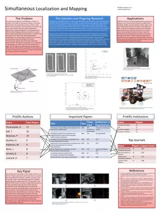
Simultaneous Localization and Mapping (SLAM). Autonomous mobile robots. autonomy. Vehicle. Actuators. Vehicle model. Sensors. Control. Vehicle autonomy. Path & motion planning. Localization. Perception. Independent from user. Localization & mapping. Independent from environment.

E N D
Autonomous mobile robots autonomy Vehicle Actuators Vehicle model Sensors Control Vehicle autonomy Path & motion planning Localization Perception Independent from user Localization & mapping Independent from environment SLAM
Introduction • In Simultaneous Localization and Mapping (SLAM) the robot does not have access to a map of the environment nor does it know its own pose. • All it is given are measurements zi:t and controls u1:t • There are 2 main forms of the SLAM problem: • Online SLAM --- estimating the posterior over the momentary pose along with the map (p(xt,m|z1:t,u1:t)) • Full SLAM---calculate a posterior over the entire pathx1:talong with the map instead of just the current pose p(x1:t,m|z1:t,u1:t) SLAM
Online SLAM It is called online SLAM since it only involves the estimation of variables that persist at time t. Many online SLAM algorithms are incremental. They discard past measurements and controls once they have been processed. SLAM
Full SLAM SLAM
Online & Full SLAM problem • In online SLAM, these integrations are typically performed one at a time. The difference between online and full SLAM has ramifications in the type of algorithms that can be used. The online SLAM problem is the result of integrating out past poses from the full SLAM problem SLAM
SLAM SLAM problems possess a continuous and discrete component. The continuous estimation problem pertains to the location of objects in the map and the robot’s own pose variables. Objects may be landmarks in feature-based representation, or they may be patches detected by range finders. The discrete nature has to do with correspondence: when an object is detected SLAM must reason about the relation of this object to previously detected objects. SLAM
Online & full SLAM and • The online posterior becomes: Taking correspondences into account the posteriors for online and full SLAM problems become: SLAM
Online & full SLAM, cont… • In practice, calculating a full posterior is usually infeasible. • Problems arise from two sources: • High dimensionality of the continuous parameter space. Many SLAM problems construct maps of tens of thousands of features and more. This involves pdfs over spaces with 105 or more. Recall in localization it was over a space of 3. • Large number of discrete correspondence variables. The number of possible assignments to the vector of all correspondence variables c1:tgrows exponentially in the time t. SLAM
SLAM with EKF The earliest SLAM algorithm is based on the Extended Kalman Filter (EKF). EKF SLAM applies the EKF to online SLAM using maximum likelihood data association. Maps in EKF SLAM are feature-based, and are composed of point landmarks. The number of point landmarks is usually less than 1000. EKF SLAM tends to work well the less ambiguous the landmarks are. SLAM
EKF SLAM EKF SLAM makes a Gaussian noise assumption for robot motion and perception. The amount of uncertainty in the posterior must be relatively small, since otherwise the linearization tend to introduce intolerable errors. EKF SLAM can only process positive sightings, it can not process negative information (absence of landmarks in sensor information) SLAM
SLAM with known correspondences This addresses only the continuous problem of SLAM Very similar to the EKF localization. Differs that it additionally estimates the coordinates of the landmarks encountered along the way (included in state vector). We will call the accumulated state vector the combined state vector yt. SLAM
SLAM with known correspondence 3N SLAM
3N-3j 3j-3 3N-3j SLAM
EKF SLAM results SLAM
EKF SLAM with unknown correspondence This type of EKF SLAM uses an incremental maximum likelihood (ML) estimator to determine correspondences. SLAM
SLAM with unknown correspondences no ct SLAM
Mahalanobis distance SLAM
Examples SLAM
MIT B21 SLAM
Feature selection & map management Gaussian noise assumption is often unrealistic, and many spurious measurements occur in the far end of the noise distribution. These measurements can cause the creation of fake landmarks (outliers) in the map, which affect the localization of the robot. The most simple technique to reject outliers is to maintain a provisional landmark list. Once a landmark has consistently been observed and its uncertainty ellipse has shrunk, it is transitioned into the regular map. SLAM
Feature selection & map management Another step, commonly found is to maintain a landmark existence probability. Such a posterior probability may be implemented as log odds ratio (denoted oj for the j-th landmark in the map). Whenever the j-th landmark mj is observed, oj is incremented by a fixed value. NOT observing mj when it is in the perceptual field of the robot sensors leads to a decrement of oj. Landmarks are removed from the map when the value oj drops below a threshold. SLAM
Numerical instability of EKF SLAM When initializing the estimate for a new landmark starting with a covariance with very large elements may induce numerical instabilities. This is because the very first covariance update step will change this value by several orders of magnitude. A better strategy involves an explicit initialization step for any feature that has not been observed before. Such a step would initialize the covariance Σt directly with the actual landmark uncertainty. SLAM
Reduce EKF brittleness The maximum likelihood approach to data association has a limitation, which arises from the fact that the maximum likelihood approach deviates from the idea of full posterior estimation in probabilistic robotics. Instead of maintaining a joint posterior over augmented states and data associations, it reduces the data association problem to a deterministic determination (treated as if MLE is always correct). Makes EKF brittle in terms of landmark confusion. Dealt with using (a) spatial arrangement, (b) signatures SLAM
Spatial arrangement • The further apart landmarks are, the smaller the chance to accidentally confuse them. • It is common practice to choose landmarks that are sufficiently far away from each other. • Trade-off: • A large # of landmarks increases the chance of confusing them. • Too few landmarks makes it more difficult to localize the robot, which in turn increases the chances of confusing them. • Therefore, researchers use intuition when selecting landmarks. SLAM
Signatures When selecting appropriate landmarks it is essential to maximize the perceptual distinctiveness of landmarks. Doors might possess different colors or corridors might have different widths. We use these as signatures. SLAM
Disadvantages of EKF SLAM A key limitation of EKF SLAM is the necessity to select appropriate landmarks. By reducing the sensor stream to the presence and absence of landmarks, a lot of sensor data is usually discarded. This leads to information loss. The quadratic update time of the EKF limits this algorithm to relatively sparse maps (<1000 features). In practice maps are in the order of 106. SLAM
Fundamental dilemma The low dimensionality cause a difficult data association problem. The fundamental dilemma of EKF SLAM: while incremental maximum likelihood data association might work well with dense maps, it tends to be brittle with sparse maps. However EKF SLAM requires sparse maps because of the quadratic update complexity. SLAM