Download
1 / 39
420 likes | 637 Views
Lecture 24. OPTIMIZATION. Optimization. Uses sophisticated mathematical modeling techniques for the analysis Multi-step process Provides improved benefit to agencies. Optimization Analysis Steps. Determine agency goals Establish network-level strategies that achieve the goals

E N D
Lecture 24 OPTIMIZATION
Optimization • Uses sophisticated mathematical modeling techniques for the analysis • Multi-step process • Provides improved benefit to agencies
Optimization Analysis Steps • Determine agency goals • Establish network-level strategies that achieve the goals • Select projects that match the selected strategies
Optimization Considerations • Other techniques are easier to understand • Loss of control perceived • Requires individuals with backgrounds in mathematics, statistics, and operations research • Consistency in data is more important • Requires sophisticated computers
Is Optimization Appropriate? • Select prioritization if: • Management wants to exercise significant control over the planning and programming exercises. • Select optimization if: • Management wants to take a global view and is willing to put substantial faith in a system.
Objective Function • Used to express an agency goal in mathematical terms • Typical objective functions • Minimize cost • Maximize benefits • Identify/define constraints
Markov Assumptions • Future condition is independent of past condition
Other Parameters • Transition costs must be defined • Life-cycle costs • Present worth analysis typically more common • Heuristic approaches reach near optimal solutions • ICB Ratio
Example of a Markov Decision Process • Assumptions • 100 mile network • Two condition states: good (1) or bad (2) • 80% of the network is in good condition • 20% of the network is in poor condition • Two maintenance activities are considered: Do Nothing (DoNo) and Overlay (Over)
Simulation Objectives • Identify the policy with the minimum expected cost after the system reaches steady state. • Establish desired long-term performance standards and minimum budgets to achieve standards or short-term objectives to reach steady state within a specified period at a minimum cost.
Markov Approach • Advantages • Disadvantages
Mathematical Programming Methods • Linear programming • Non-linear programming • Integer programming • Dynamic programming
Variable Number 2 Objective Functions Feasible Solutions Constraints Variable Number 1 Linear Programming
Variable Number 2 Objective Functions Feasible Solutions Variable Number 1 Non-linear Programming Constraints
Decision Flow 5 A 5 3 3 Begin 6 B End 4 2 2 (Costs) C 6 Solution Flow Dynamic Programming
Selecting the Appropriate Programming Method • Function of: • Type of variables in analysis • Form of objective function • Sequential nature of decisions • Typical approaches: • Linear programming most common • Dynamic programming second most common approach • Non-linear third most common approach • No agency is using integer programming
Markov Implementation Steps • Define road categories • Develop condition states • Identify treatment alternatives • Estimate transition probabilities for categories and alternatives
Markov Implementation Steps (cont.) • Estimate costs of alternatives • Calibrate model • Generate scenarios • Document models • Update models
Case Study - Kansas DOT • System Components • Network optimization system (NOS) • Project optimization system (POS) (was not fully operational in 1995) • Pavement management information system (PMIS)
Overview of KDOT Data Collection Activities • Collect pavement distress information • Monitor rutting • Collect roughness data
KDOT M&R Programs • Major Modification Program • Substantial Maintenance Program
KDOT Databases • CANSYS • PMIS
KDOT NOS Analysis • 216 possible condition states • Primary influence variables: • Indices to appearance of distress • Rate of change in distress • Rehabilitation actions based on one of 27 distress states • Linear programming used to develop programs to maintain acceptable conditions for lowest possible cost
KDOT POS Analysis • Projects from NOS are investigated in more detail using POS • Identify initial designs to maximize user benefits
KDOT System Development • Issue paper • PMS Steering Committee • Pavement Management Task Force • Consultant
Instructional Objectives • Understand philosophy of optimization • Identify concepts involved in optimization analysis • Identify types of models used in optimization analysis