Download
1 / 59
590 likes | 700 Views
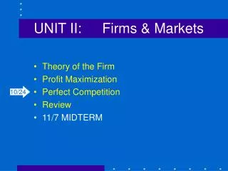
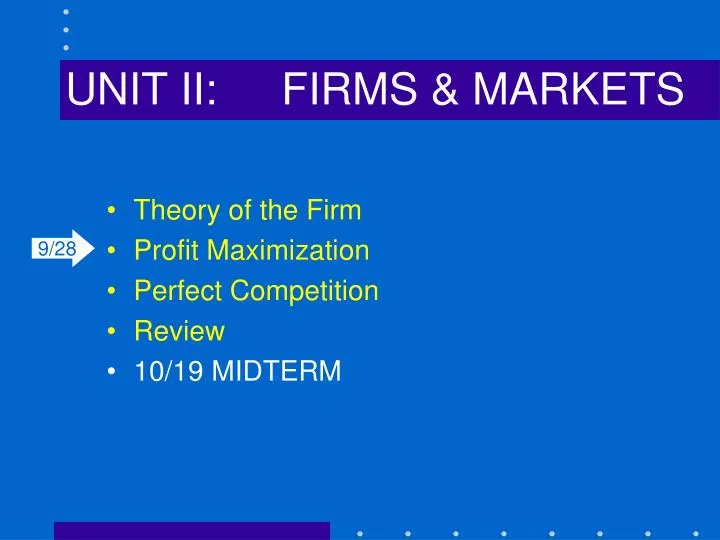
UNIT II: FIRMS & MARKETS. Theory of the Firm Profit Maximization Perfect Competition Review 10 /19 MIDTERM. 9/ 28. Profit Maximization . Last Time The Short-Run and the Long-Run Firm and Market Supply Perfect Competition (Part 1). Last Time.

E N D
UNIT II: FIRMS & MARKETS • Theory of the Firm • Profit Maximization • Perfect Competition • Review • 10/19 MIDTERM 9/28
Profit Maximization • Last Time • The Short-Run and the Long-Run • Firm and Market Supply • Perfect Competition (Part 1)
Last Time We saw last time that we can solve the firm’s cost minimization problem analogously to the consumer’s utility maximization problem. Cost minimization requires that the firm produce using a combination of inputs for which the ratios of the marginal products, or the marginal rate of technical substitution, equals the ratio of the input prices: MRTS = w/r • 2 Provisos: • Only in the Long-Run • Only part of the firm’s problem
Profit Maximization The firm wants to maximize this difference: Profit (P) = Total Revenue(TR) – Total Cost(TC) TR(Q) = PQ TC(Q) = rK + wL P Price L Labor Q Quantity K Capital w Wage Rate r Rate on Capital Q = f(K,L) Revenue Cost
Profit Maximization Profit (P) = Total Revenue(TR) – Total Cost(TC) $ Consider a firm with long-run total costs TC. TC Q1 Q2 Q3Q
Profit Maximization Profit (P) = Total Revenue(TR) – Total Cost(TC) $ To maximize profits, the firm finds Q where distance between TC and TR is greatest. the same slope. TR = PQ TC Q1 Q2 Q3Q
Profit Maximization Profit (P) = Total Revenue(TR) – Total Cost(TC) $ To maximize profits, the firm finds Q where distance between TC and TR is greatest.same slope. TC TR = PQ Q1 Q2 Q3Q
Profit Maximization Profit (P) = Total Revenue(TR) – Total Cost(TC) $ To maximize profits, the firm finds Q where distance between TC and TR is greatest.same slope. TC TR = PQ Q1 Q2 Q Q
Profit Maximization Profit (P) = Total Revenue(TR) – Total Cost(TC) $ To maximize profits, the firm finds Q where distance between TC and TR is greatest. This will be where they have the same slope.. slope. TR = PQ Pmax TC Q1 Q Q* Q
Profit Maximization Marginal Analysis: If TC is rising faster than TR, reduce Q. If TR is rising faster than TC, increase Q. Profit (P) = Total Revenue(TR) – Total Cost(TC) $ TR = PQ Pmax TC Q1 Q Q* Q
Profit Maximization Marginal Analysis: Recall: slope TR = MR slope TC = MC Hence, to maximize profits: MR = MC Profit (P) = Total Revenue(TR) – Total Cost(TC) $ TR = PQ Pmax TC Q1 Q Q* Q
Profit Maximization The firm wants to maximize this difference: Profit (P) = Total Revenue(TR) – Total Cost(TC) TR(Q) = PQ TC(Q) = rK + wL P Price L Labor Q Quantity K Capital w Wage Rate r Rate on Capital Q = f(K,L) Revenue Cost
Last time: we considered a firm that produces output according to the following production function. Q = 4K½L½ and w = $18 and r = $36. How much will it cost this firm to produce 10 units of output in the long-run? Q units? The long-run total cost curve (TC(Q)) represents the minimum cost to produce Q units of output. Profit Maximization
Cost Minimization in the Long-Run How much will it cost this firm to produce Q units of output in the long-run? Q = 4K1/2L1/2 w = 18; r = 36 MRTS = MPL/MPK MPL = 2K1/2L-1/2 MPK = 2K-1/2L1/2 MRTS = K/L. = w/r = 18/36 = L = 2K. The firm’s optimal factor proportion (given technology and factor prices).
Cost Minimization in the Long-Run How much will it cost this firm to produce Q units of output in the long-run? Q = 4K1/2L1/2 L = 2K => Q = 4K1/2(2K)1/2 = 4(2)1/2K • K = Q/[4(2)1/2]; L = Q/[2(2)1/2] TC(Q) = wL + rK TC(Q) = 18(Q/[2(2)1/2]) + 36(Q/[4(2)1/2]) = 9Q/(2)1/2 + 9Q/(2)1/2
Cost Minimization in the Long-Run How much will it cost this firm to produce Q units of output in the long-run? TC = 9Q/(2)1/2 + 9Q/(2)1/2 = 18/(2)1/2(Q) = 12.73Q MC = 12.73 = AC K K* We can solve for the firm’slong run total cost function for any level of output. Q = 10
Profit Maximization Demand for the firm’s output is given by Q = 100 – 2P. Find the firm’s profit maximizing level of output. Q = 4K1/2L1/2 w = 18; r = 36 Q = 100 – 2P => P = 50 – 1/2Q TR = PQ = (50 – 1/2Q)Q = 50Q – 1/2 Q2 MR = 50 – Q = MC = 12.73 => Q* = 37.27; P* = 31.37
Profit Maximization Demand for the firm’s output is given by Q = 100 – 2P. Find the firm’s profit maximizing level of output. Q = 4K1/2L1/2 w = 18; r = 36 Q = 100 – 2P => P = 50 – 1/2Q TR = PQ = (50 – 1/2Q)Q P = TR – TC = 50Q – 1/2 Q2 – 12.73Q FOC: dP/dQ = 50 – Q – 12.73 = 0 => Q* = 37.27; P* = 31.37
Profit Maximization in the Long-Run We solved the firm’s optimization problem focusing on the profit output level, Q*, but it is important to emphasize that the optimization principle also tell us about input choices. When the firm chooses an output level Q* that maximizes P for given factor prices (w, r), the firm has simultaneously solved for L* and K*. To produce Q* = 37.27 (given the production function, Q = 4K1/2L1/2, and optimal factor proportion, L = 2K), we find: L* = 6.58; K* = 3.29. Finally, P = TR–TC = PQ–12.73Q = (31.37–12.73)37.27 = $694.71.
Profit Maximization in the Short-Run We saw that the firm maximizes profit by choosing a level of output such that marginal revenue equals marginal cost MR = MC. In the long-run, this implies that the firm will be utilizing its optimal factor proportion, such that MRTS = w/r. In the short-run, however, K is fixed, so the firm will not be able to optimally adjust factor proportions. Does the firm maximize profits by setting MR = MC in the short-run? How?
Profit Maximization in the Short-Run We solved the firm’s optimization problem focusing on the output level, but it is important to emphasize that the optimization principle also tell us about input choices. When the firm chooses an output level (Q*) that maximizes profit for given factor prices (w, r), the firm has simultaneously solved for L* and K*. In the short-run, the firm also maximizes P by setting MR = MC.But because K is fixed, the problem is simply one of optimal utilization of labor. In other words, the firm asks, “On the margin, can I increase my profit by adding (or subtracting) another unit of labor from the production process?”
Profit Maximization in the Short-Run Q = 4K1/2L1/2 w = 18; r = 36 K = 16 P = 10 MR = MC TR = PQ = 10Q TC = rK + wL = 36(16) + 18L
Profit Maximization in the Short-Run Q = 4K1/2L1/2 w = 18; r = 36 K = 16 P = 10 MR = MC TR = PQ = 10Q TC = rK + wL = 36(16) + 18L [ Q = 16L½ => L = (Q/16)2 ] TC = 36(16) + 18(Q/16)2 = 576 + 18(Q/16)2 MR = 10 = MC = (36/256)Q => Q = 71.1; L = 19.8 Revenue Cost
Profit Maximization in the Short-Run In the short-run, the firm’s profit maximizing calculus weighs the benefit of hiring an additional unit of labor versus its cost. If the firm can add (subtract) another unit of labor and increase revenue by more than it increases cost, it should add (subtract) it, and it should keep on adding (subtracting) until MR = MC.
Profit Maximization in the Short-Run What does an additional unit of L contribute to P? First, hiring an additional unit of L increases the firm’s output (Q) By how much? MPL = dQ/dL. MRPL = dTR = P dQ dL dL = P (MPL) Marginal Revenue Product (MRP) The dollar amount added to revenue from an additional unit of labor (capital). For a Price-taker this can be rewritten as:
Profit Maximization in the Short-Run What does an additional unit of L contribute to P? But hiring an additional unit of L also increases the firm’s total costs. MFCL= w Marginal Factor Cost (MFC) The dollar amount added to total cost from an additional unit of labor (capital). NOTE (for fixed K): MC = dTC/dQ = w (dL/dQ) MC = w (1/MPl)
Profit Maximization in the Short-Run So the firm’s short-run optimality condition can be rewritten as: MRPL = MFCL If the firm can add (subtract) another unit of labor and increase revenue by more than it increases cost, it should add (subtract) it, and it should keep on adding (subtracting) until MRPL = MFCL. This, in turn, is what determines the firm’s (short-run) demand for labor: P (MPL) = w
Profit Maximization in the Short-Run Consider a price-taking firm that is currently producing 450 units of output at a price of $2.50 per unit. In the short run, the firm’s capital stock is fixed at 16 machine-hours. The firm is currently employing 100 hours of labor at a wage of $10/hour, and the at a rental rate (r) is $10/hour. With this mix of inputs MPK=2 and MPL= 4. Is the firm maximizing profits in the short run?
Profit Maximization in the Short-Run Is the firm maximizing profits in the short run? Yes. MRPL = P(MPL) = 2.50(4) = 10 = w = MFCL MR = P = $2.50; MC = w/MPL = $10/4 = $2.50 Does it matter that MPL/MPK = w/r (4/2 = 10/10) ? Does it matter that P = TR-TC = 1125 – 1160 = -35 ? Shut down rule: If P < AVC, Q = 0. The firm would lose its fixed costs ($160) if it shut down, or $35 if it produces Q = 450. What matters is variable costs, because fixed costs are spent (“sunk”) in the short run. Profit max = Loss min.
Supply in the Short-Run TC P = TR – TC = 0 PRICE TAKER P = MR $ $ TR At price Po, the firm earns 0 profit. Q MC AC P = MR Q* Q
Supply in the Short-Run TR TC P = TR – TC > 0 PRICE TAKER P = MR $ $ If the price rises … Output rises … Q MC AC P = MR Q Q
Supply in the Short-Run TR TC P = TR – TC > 0 PRICE TAKER P = MR $ $ If the price rises … And the firm earns profit Q MC AC P = MR Q Q
Supply in the Short-Run TC P = TR – TC < 0 PRICE TAKER P = MR $ $ If the price decreases… Output falls TR Q MC AC P = MR Q Q
Supply in the Short-Run TC P = TR – TC < 0 PRICE TAKER P = MR $ $ If the price decreases… And the firm has losses TR Q MC AC P = MR Q Q
Supply in the Short-Run TC P = TR – TC < 0 PRICE TAKER P = MR $ $ The firm will continue to produce (< Q*) iff P > AVC … Losses are less than fixed costs. TR Q MC AC AVC P = MR Q
Supply in the Short-Run TR TC P = TR – TC < 0 PRICE TAKER P = MR $ $ The firm’s short-run supply curve is in orange Where MR = MC and P > AVC. Q MC AC AVC Q
Supply in the Long-Run In the short run, firms adjust to price signals by varying their utilization of labor (variable factors). In the long-run, firms adjust to profit signals by • varying plant size (fixed factors); and • entering or exiting the market. What determines the number offirms in the long-run?
Supply in the Long-Run Short-run equilibrium with three firms. Firm A is making positive profits, Firm B is making zero profits, and Firm C is making negative profits (losses). q: firm Q: market MC MC $ P MC AC AC AC q q q Firm A Firm B Firm C
Supply in the Long-Run Short-run equilibrium with three firms. Firm A is making positive profits, Firm B is making zero profits, and Firm C is making negative profits (losses). MC MC $ P MC AC AC AVC AC q q q Firm A Firm B Firm C
Supply in the Long-Run Short-run equilibrium with three firms. Firm A is making positive profits, Firm B is making zero profits, and Firm C is making negative profits (losses). In the long run, Firm C will exit the market. MC $ P MC AC AC q q q Firm A Firm B Firm C
Supply in the Long-Run In the long-run, inefficient firms will exit, and new firms will enter, as long as some firms are making positive economic profits. MC $ P MC MC AC AC AC q q q Firm A Firm B Firm D
Supply in the Long-Run In the long-run, if there are no barriers to entry, then new firms have access to the most efficient productiontechnology. We call this the efficient scale. $ P* MC MC MC AC AC AC q* q q* q q* q Firm A Firm D Firm E
Supply in the Long-Run The long-run supply curve. P* is the lowest possible price associated with non-negative profits, P* = ACmin. s1=(mc1) s2 Sn, where n is the number of firms in the market. $ P* s3 s4 Q
Supply in the Long-Run The long-run supply curve. We can eliminate portions of the individual firms’ supply curves below P* (firms will exit). s1 s2 $ P* s3 s4 Q
Supply in the Long-Run The long-run supply curve. We can also eliminate portions of the individual firms’ supply curves above P* (demand will be met by another firm’s supply curve). s1 s2 $ P* s3 s4 Q
Supply in the Long-Run The long-run supply curve. As the number of firms increases, the long run supply curve approximates a straight line at P* = ACmin. $ ACmin = P* LRS Q
Supply in the Long-Run Long-run equilibrium. Firms are producing at the efficient scale. P* = ACmin; P = 0. $ $ P* MC AC LRS D q* q Q* Q
Perfect Competition • Perfect Competition • Equilibrium and Efficiency • General Equilibrium • Welfare Analysis
Perfect Competition Assumptions • Firms are price-takers: can sell all the output they want at P*; can sell nothing at any price > P*. • Homogenous product: e.g., wheat, t-shirts, long-distance phone minutes. • Perfect factor mobility: in the long run, factors can move costlessly to where they are most productive (highest w, r). • Perfect information: firms know everything about costs, consumer demand, other profitable opportunities, etc.
Perfect Competition Implications • Firms earn zero (economic) profits. • Price is equal to marginal cost. • Firms produce at minimum average cost, i.e., “efficient scale.” • Market outcome is Pareto-efficient.