Download
1 / 44
440 likes | 446 Views
Plantwide control: Towards a systematic procedure. Sigurd Skogestad Department of Chemical Engineering Norwegian University of Science and Tecnology (NTNU) Trondheim, Norway Plenary Presentation at ESCAPE’12, den Haag, May 2002.

E N D
Plantwide control: Towards a systematic procedure Sigurd Skogestad Department of Chemical Engineering Norwegian University of Science and Tecnology (NTNU) Trondheim, Norway Plenary Presentation at ESCAPE’12, den Haag, May 2002
Personal anecdote from Jack Ponton, University of Edinburgh (1993) ”Some years ago, when a fairly junior academic, he took an industrial sabattical. Having told that he was a teacher of process control, he was presented with a process flowsheet and asked to put control loops on it. Despite having taught process control – including differential eqautions, Laplace tranforms, Bode diagrams and so on – he was at loss even as to start the task. And so most have been generations before of chemical engineering graduates. And this is the control task which process engineers in industry are most frequently called upon to perform.”
Practice I: Tennessee Eastman challenge problem (Downs, 1991)
Alan Foss (“Critique of chemical process control theory”, AIChE Journal,1973): The central issue to be resolved ... is the determination of control system structure. Which variables should be measured, which inputs should be manipulated and which links should be made between the two sets?
Plantwide control • Not the tuning and behavior of each control loop, • But rather the control philosophy of the overall plant with emphasis on the structural decisions: • Selection of manipulated variables (“inputs”) • Selection of controlled variables (“outputs”) • Selection of (extra) measurements (extra outputs) • Selection of control configuration (structure of overall controller that interconnects the controlled, manipulated and measured variables) • Selection of controller type (PID, decoupler, MPC etc.). • That is: All the decisions made before we get to “Ph.D” control
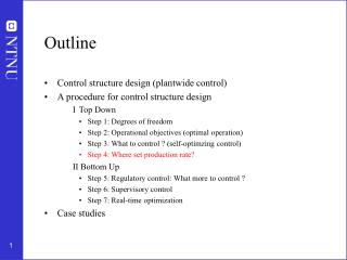
Outline • Plantwide control procedure • Top-down definition of objectives • What to control I: Primary controlled variables • Inventory control - where set production rate • Bottom-up assignment of control loops • What to control II: Secondary controlled variables • Decentralized versus multivariable control in supervisory layer
Related work • Page Buckley (1964) - Chapter on “Overall process control” (still industrial practice) • Alan Foss (1973) - control system structure • George Stephanopoulos and Manfred Morari (1980) • Bill Luyben and coworkers (1975- ) – many “snowball effect” • Ruel Shinnar (1981- ) - “dominant variables” • Jim Douglas and Alex Zheng (Umass) (1985- ) • Jim Downs (1991) - Tennessee Eastman process • Larsson and Skogestad (2000): Review of plantwide control
Stepwise procedure plantwide control I. TOP-DOWN Step 1. DEFINE OVERALL CONTROL OBJECTIVE Step 2. DEGREE OF FREEDOM ANALYSIS Step 3. WHAT TO CONTROL? (primary variables) Step 4. PRODUCTION RATE Steady-state considerations: No control knowledge required!
II. BOTTOM-UP (structure control system): Step 5. REGULATORY CONTROL LAYER 5.1 Stabilization (including level control) 5.2 Local disturbance rejection (inner cascades) What more to control? (secondary variables) Step 6. SUPERVISORY CONTROL LAYER Decentralized or multivariable control (MPC)? Pairing? Step 7. OPTIMIZATION LAYER (RTO)
Step 1. Overall control objective • What are the operational objectives? • Quantify: Minimize scalar cost J • Usually J = economic cost [$/h] • + Constraints on flows, equipment constraints, product specifications, etc.
Step 2. Degree of freedom (DOF) analysis • Nm : no. of dynamic (control) DOFs (valves) • Nss = Nm- N0 : steady-state DOFs • N0 : liquid levels with no steady-state effect (N0y)+ purely dynamic control DOFs (N0m) Cost J depends normally only on steady-state DOFs
Distillation column with given feed Nm = 5, N0y = 2, Nss = 5 - 2 = 3 (2 with given pressure)
Alternatives structures for optimizing control Step 3: What should we control?
Step 3. What should we control? (primary controlled variables) • Intuition: “Dominant variables” (Shinnar) • Systematic: Define cost J and minimize w.r.t. DOFs • Control active constraints (constant setpoint is optimal) • Remaining DOFs: Control variables c for which constant setpoints give small (economic) loss Loss = J - Jopt(d) when disturbances d occurs
Self-optimizing control(Skogestad, 2000) Loss L = J - Jopt (d) Self-optimizing control is achieved when a constant setpoint policy results in an acceptable loss L (without the need to reoptimize when disturbances occur)
Application: Recycle processJ = V (minimize energy) 5 4 1 Given feedrate F0 and column pressure: 2 3 Nm = 5 N0y = 2 Nss = 5 - 2 = 3 Max. reactor volume, xB > 0.98
Recycle process: Selection of controlled variables • Step 3.1 J=V (minimize energy with given feed) • Step 3.1 DOFs for optimization: Nss = 3 • Step 3.3 Most important disturbance: Feedrate F0 • Step 3.4 Optimization: Constraints on max. Mr and xB always active • Step 3.5 1 DOF left,candidate controlled variables: F, D, L, xD, ... • Step 3.6 Loss with constant setpoints. Good: xD, L/F. Poor: F, D, L
Recycle process: Loss with constant setpoint, cs Large loss with c = F (Luyben rule) Negligible loss with c = L/F
Recycle process: Proposed control structurefor case with J = V (minimize energy) Active constraint Mr = Mrmax Active constraint xB = xBmin
Recycle systems: Do not recommend Luyben’s rule of fixing a flow in each recycle loop (even to avoid “snowballing”)
Good candidate controlled variables c (for self-optimizing control) Requirements: • The optimal value of c should be insensitive to disturbances • c should be easy to measure and control • The value of c should be sensitive to changes in the steady-state degrees of freedom (Equivalently, J as a function of c should be flat) • For cases with more than one unconstrained degrees of freedom, the selected controlled variables should be independent. Singular value rule (Skogestad and Postlethwaite, 1996): Look for variables that maximize the minimum singular value of the appropriately scaled steady-state gain matrix G from u to c
Step 4. Where set production rate? • Very important! • Determines structure of remaining inventory (level) control system • Set production rate at (dynamic) bottleneck • Link between Top-down and Bottom-up parts
Production rate set at inlet :Inventory control in direction of flow
Production rate set at outlet:Inventory control opposite flow
Reactor-recycle process:Given feedrate with production rate set at inlet
MAX Reactor-recycle process:Reconfiguration required when reach bottleneck (max. vapor rate in column)
Reactor-recycle process:Given feedrate with production rate set at bottleneck (column) F0s
II. Bottom-up assignment of loops in control layer • Identify secondary (extra) controlled variable • Determine structure (configuration) of control system (pairing) • A good control configuration is insensitive to parameter changes! Industry: most common approach is to copy old designs
y1 = c y2 = ? Step 5. Regulatory control layer • Purpose: “Stabilize” the plant using local SISO PID controllers to enable manual operation (by operators) • Main structural issues: • What more should we control? (secondary cv’s, y2) • Pairing with manipulated variables (mv’s)
Selection of secondary controlled variables (y2) • The variable is easy to measure and control • For stabilization: Unstable mode is “quickly” detected in the measurement (Tool: pole vector analysis) • For local disturbance rejection: The variable is located “close” to an important disturbance (Tool: partial control analysis).
Primary controlled variable y1 = c (supervisory control layer) Local control of y2 using u2 (regulatory control layer) Setpoint y2s : new DOF for supervisory control Partial control
Step 6. Supervisory control layer • Purpose: Keep primary controlled outputs c=y1 at optimal setpoints cs • Degrees of freedom: Setpoints y2s in reg.control layer • Main structural issue:Decentralized or multivariable?
Decentralized control(single-loop controllers) Use for: Noninteracting process and no change in active constraints + Tuning may be done on-line + No or minimal model requirements + Easy to fix and change - Need to determine pairing - Performance loss compared to multivariable control - Complicated logic required for reconfiguration when active constraints move
Multivariable control(with explicit constraint handling - MPC) Use for: Interacting process and changes in active constraints + Easy handling of feedforward control + Easy handling of changing constraints • no need for logic • smooth transition - Requires multivariable dynamic model - Tuning may be difficult - Less transparent - “Everything goes down at the same time”
Step 7. Optimization layer (RTO) • Purpose: Identify active constraints and compute optimal setpoints (to be implemented by supervisory control layer) • Main structural issue: Do we need RTO? (or is process self-optimizing)
Conclusion Procedure plantwide control: I. Top-down analysis to identify degrees of freedom and primary controlled variables (look for self-optimizing variables) II. Bottom-up analysis to determine secondary controlled variables and structure of control system (pairing).
More details.... • Skogestad, S. (2000), “Plantwide control -towards a systematic procedure”, Proc. ESCAPE’12 Symposium, Haag, Netherlands, May 2002. • Larsson, T., 2000. Studies on plantwide control, Ph.D. Thesis, Norwegian University of Science and Technology, Trondheim. • Larsson, T. and S. Skogestad, 2000, “Plantwide control: A review and a new design procedure”, Modeling, Identification and Control, 21, 209-240. • Larsson, T., K. Hestetun, E. Hovland and S. Skogestad, 2001, “Self-optimizing control of a large-scale plant: The Tennessee Eastman process’’, Ind.Eng.Chem.Res., 40, 4889-4901. • Larsson, T., M.S. Govatsmark, S. Skogestad and C.C. Yu, 2002, “Control of reactor, separator and recycle process’’, Submitted to Ind.Eng.Chem.Res. • Skogestad, S. (2000). “Plantwide control: The search for the self-optimizing control structure”. J. Proc. Control10, 487-507. See also the home page of Sigurd Skogestad: http://www.chembio.ntnu.no/users/skoge/