Download
1 / 73
740 likes | 891 Views
& Mathematical Institute, Leiden University. (formerly ADN ) IIASA. VEOLIA- Ecole Poly- technique. The canonical equation of adaptive dynamics. a new role for the effective population sizes of population genetics. Hans (= J A J * ) Metz. Preamble .

E N D
& Mathematical Institute, Leiden University (formerly ADN) IIASA VEOLIA- Ecole Poly- technique The canonical equationof adaptive dynamics a new role for the effective population sizes of population genetics Hans (=JAJ*) Metz
Preamble Real evolution mostly takes place in higher (even infinite) dimensional trait spaces. In higher dimensions the main ideas introduced by means of the graphical constructions still apply, but the analysis of the monomorphic dynamics hinges the ordering properties of the real line. To study the dynamics in the higher dimensional case we ususally fall back on a differential equation, grandly called the Canonical Equation of adaptive dynamics. Goal: This talk is given to its derivation, and to an unexpected recently discovered link with the theory of random genetic drift.
the ecological theatre and the evolutionary play Long term adaptive evolution proceeds through the continual filtering of new mutations by selection. The supply of new phenotypes by mutation depends on the genotypic architecture and the genotype to phenotype map. Selection is a population dynamical process. Convenient idealisation: The time scales of the production of novel variation and of gene substitutions are separated.
the adaptive play Given a population dynamics one can graft onto it an adaptive dynamics: Just assume that individuals are characterised by traits that may change through mutation, and that affect their demographic parameters. The speed of adaptive evolution is proportional tothe population size n.
a second, silent, play: random genetic drift Given a population dynamical model one can also graft onto it a random genetic drift. Just imagine that each individual harbours two alleles without consequential phenotypic effect, which in the reproductive process are reassorted according to Mendel’s laws. The speed at which variation is lost over time is inverselyproportional to n.
The product of this constant and n is known as the effective population sizene. a formal connection between the two plays Result: The constants that appear in front of n in the formulas for the speeds of adaptive evolution and random genetic drift are the same.
the population dynamical side of adaptive evolution Adaptive evolution occurs by the repeated substitution of mutants in largish populations. Mutants emerge single in an environment set by a resident population. How many mutants occur per time unit depends on the size of the resident birth stream. The mutant invasion process depends on their phenotype and on the environment in which they invade. The assumption that the resident population is large makes that both the birth stream and the environment can be calculated from a deterministic community model.
modelling the ecological theatre The easiest way of accomodating all sort of life history detailin a single overarching formalism is to do the population dynamical bookkeeping from births to births. (C.f. Lotka’s integral equation.) • By allowing multiple birth states it is moreover possible to accommodate i.a. • parentally mediated differences in offspring size, social status, etc. • spatially distributed populations (use location as birth state component) • cyclic environments (use phase of cycle as birth state component) • genetic sex determination, including haplo-diploid genetics, etc • genetic polymorphisms. • I will proceed as if the number of possible birth states is finite.
Odo Diekmann Mats Gyllenberg Equilibria of structured populations generally satisfy: B= L(X|EX)B, EX=F(I), I=G(X|EX)B modelling the ecological theatre Diekmann, Gyllenberg & Metz (2003) TPB 63: 309-338 trait vector (affects the two operators that describe individual behaviour)
Odo Diekmann Mats Gyllenberg Equilibria of structured populations generally satisfy: B= L(X|EX)B, EX=F(I), I=G(X|EX)B modelling the ecological theatre equilibrium Birth rate vector per unit of area environmental input, i.e., the Environment as perceived by the individuals per capita lifetime impingement on the environment next generation operator (i.e., lij is the Lifetime number of births in state i expected from a newborn in state j) population output, i.e., Impingement on the environment
Odo Diekmann Mats Gyllenberg Equilibria of structured populations generally satisfy: B= L(X|EX)B, EX=F(I), I=G(X|EX)B modelling the ecological theatre equilibrium Birth rate vector per unit of area result of the dynamic equilibrium of the surrounding community environmental input, i.e., the Environment as perceived by the individuals next generation operator (i.e., lij is the Lifetime number of births in state i expected from a newborn in state j)
branching (concentrate on traits, and rescale time appropriately) two subsequent limits individual-based stochastic process t trait value mutational step size 0 system size ∞ successful mutations/time 0 limit type:
the canonical equation The “canonical equation of adaptive dynamics” was derived to describe the evolution of quantitative traits in realistic ecologies. Assumptions: large population sizes, mutation limitation, small mutational steps. * *and, initially, simple ODE population models
the canonical equation X: value of trait vector predominant in the population n: population size, : mutation probability per birth event C: mutational covariance matrix, s: invasion fitness, i.e., initial relative growth rate of a potential Y mutant population.
basic ideas and first derivation (1996) hard proofs (2003) extensions (2008) Ulf Dieckmann & Richard Law Nicolas Champagnat & Sylvie Méléard Michel Durinx & me hard proof for pure age dependence Chi Tran (2006) history Mendelian diploids general life histories discrete generations with Poisson # offspring only rigorous for ODE model general case not yet published Underlying assumptions rather unbiological: individuals reproduce clonally, have exponentially distributed lifetimes and give birth at a constant rate from birth onwards (i.e., an ODE population model). so far only for community equilibria non-rigorous
an unexpected connection Part III will argue, based on conjectured extensions of theorems that have been proven for simple special cases, that ne,A=ne,D the effective population size for random genetic Drift.
derivation of the canonical equation mean of [mutational step approximation for the probability that a Y-mutant invades] B=bU, 1TU=1 births per unit of time probability of mutation per birth event For general equilibrium population dynamics the canonical equation appears first in another form: approximation for the evolution is mutation limited mutational steps are small
R0(Y|EX) average life-time offspring numberof a mutant allele producing Y when singly substituted in the resident genotype * demographic ingredients 1 ( calculated as dominant eigenvalue of a next generation operator L(Y|EX) ). For the resident:R0(X|EX) = 1. Ustable birth state distribution of resident( allele)s , normalised dominating right eigenvector of L(X|EX), 1TU =1, V(birth rate based) reproductive values of newborn resident( allele)s, co-normalised dominating left eigenvector of L(X|EX), VTU = 1.
* with mi the lifetime number of offspring born in state i, begotten by a resident allele born in state j. demographic ingredients 2 For the resident:R0(X|EX) = 1. Ustable birth state distribution of resident( allele)s , normalised dominating right eigenvector of L(X|EX), 1TU =1, V(birth rate based) reproductive values of newborn resident( allele)s, co-normalised dominating left eigenvector of L(X|EX), VTU = 1.
1000 individuals # 100 10 time 1 10 20 0 Ilan Eshel J.B.S. Haldane from the theory of branching processes In an ergodic environmentEX a population starting from a single individual: either goes extinct, with probabilityQ(Y|EX), or "grows exponentially" at a relative rates(Y|X). For constant EX and smalls:
Brook Taylor the average effective step approximation for the probability that a Y-mutant invades probability density of mutational steps Z = Y-X Smooth genotype to phenotype maps lead to locally additive genetics. In diploids the mutational effect doubles over a full substitution on the stronger assumption that the mutations distribution is symmetric around the resident C on the assumption that mutations are unbiased mutational covariance matrix
regulatory regions coding region DNA reading direction aside on genotype to phenotype maps Some evo-devo: Genotype to phenotype maps are treated as smooth maps from some vector space of gene expressions to some vector space of phenotypes. Rationale: Most phenotypic evolution is probably regulatory, and hence quantitative on the level of gene expressions.
the genotype to phenotype map: Consider a representative locus, to be called A, affecting the phenotypic trait, with resident allele a and potential mutant A. Alleles are supposed to affect the phenotype in a quantitative manner, expressible through an allelic trait Xaresp. XA . The corresponding phenotypes will be written as Xaa,XaA,XAA: Xaa=( ;Xa,Xa;), XaA=( ;Xa,XA;),XAA=(;XA,XA;), with subject to the restriction ( ;Xa,XA;)=( ;XA,Xa;) ( no parental effects).
The symmetry restriction implies ∂(;Xa,XA;)∂(;Xa,XA;) ∂XaXA=Xa∂XAXA=Xa = :=A´( ;Xa,Xa;) XAA local approximate additivity Andrea Pugliese Tom van Dooren We assume to be sufficiently smooth, and express the smallness of the allelic effect asXA = Xa + Z. Hence XaA=( ;Xa,Xa;) + A´( ;Xa,Xa;)Z +O(2) XAA=(;Xa,Xa;)+A´(;Xa,Xa;)Z+A´(;Xa,Xa;)Z+O(2) = ( ;Xa,Xa;)+2 A´( ;Xa,Xa;)Z+O(2).
Assume that the total mutational change is not only small but also unbiased, i.e, then the mutational covariance matrix Let, given that a mutation happens, the probability that this mutation happens at theA-locus be pA,and let the distribution of the mutational step,Y:=XA-Xa, befA .
mutational covariances need not be constant! In the Mendelian case the derivation from the basic ingredients, genotype to phenotype map and genotypic mutation structure, shows that the canonical equation represents but the lowest level in a moment expansion. The next level is a differential equation for change of the mutational covariance matrix, depending on mutational 3rd moments, etc.
recovering population size and fitness Tr : average age at giving birth, of the residents. Ts : average survival time
* withfi(a) the probability density of the age at death of an individual born in state i. * with(a)composed of the average pro capita birth rates at agea. demographic ingredients 3
aside: robustness of the CE Géza Meszéna For small mutational stepsthe influence of the mutants on the environment at higher densities comes in only as a term with a higher order in the mutational step size than the terms accounted for by the canonical equation. Whether or not some previous mutants have not yet gone to fixation has little influence on the invasion of new mutants. The applicability of the canonical equationextends well beyond the case of strict mutation limitation.
random genetic Drift Operational definition: The effective population size for random genetic Drift, ne,D, is most easily defined as the parameter occurring in the usual diffusion approximation for the temporal development of the probability density of the frequency p of a neutral gene. Interpretation: The size of a population with non-overlapping generations and multinomial pro capita off-spring numbers that produces the same (asymptotic) decay of genetic variability as the focal population.
Proposition The effective population sizes ne,Afor Adaptive evolution and ne,Dfor random genetic Drift are equal whatever the life history or ecological embedding.
idea of the proof Connect the approximation formula for the invasion probability derived from branching process theory (Eshel’s formula) with the probability for take-over for a diffusion approximation including selection, : initial frequency of mutant allele selection coefficient • Why this particular combination of limits ? • Why this formula for the initial mutant allele frequency p0? • Why this formula for the selection coefficient s? proxy for system size ~
idea of the proof ~ Why this formula for the selection coefficient s ? In the diffusion approximation time is measured in generations. Hence s = Tr s . ~
idea of the proof Why this particular combination of limits ? ne,D n reflects the behavioural laws of resident individuals. We want to determine the first order term for small positive s in the Taylor expansion of the invasion probability. We want to remove the effect of the finiteness of n.
idea of the proof p0 Why this particular combination of limits ? Left and right we take subsequent limits in different ways: (1) from full population dynamics to branching process, followed by an approximation for the invasion probability, (2) from full population dynamics to diffusion process, followed by a two-step approximation for the invasion probability. To get equality we want the corresponding paths in parameter space to approach the eventual limit point from the same direction.
idea of the proof Why this formula for the initial mutant allele frequency p0 ?
belief Order the states such that the birth states come first. Then the next generation operator L(X,EX ) can be expressed as with Any relevant life history process can be uniformly approximated by finite state processes. In continuous time at population dynamical equilibrium (E = EX) : B: individual level state transition generator A: average birth rate operator
idea of the proof The genetic diffusion for a structured population consists of a slow diffusion of the gene frequency p, preceded by a fast process bringing the population state the stationary population state without genetic differentiation, For the fast process results in : co-normalised left eigenvector of A+B to with the normalised eigenvector of A+B. Why this formula for the initial mutant allele frequency p0 ?
idea of the proof For a just appeared mutant: Lemma: Why this formula for the initial mutant allele frequency p0 ? For the fast process results in : co-normalised left eigenvector of A+B
a corollary: individual-based calculation of ne,D William G Hill Edward Pollak a result already reached by different means by WilliamGHill (1972) for the simple age-dependent case, and by Edward Pollak (1979, ...) for the age dependent case with multiple birth states.
a practical consequence At equal genetic and developmental architectures and population dynamical regimesthe speeds of adaptive evolution and random genetic drift are inversely proportional. Already for moderately large effective population sizesadaptive processes dominate, and neutral substitutions will be largely caused by genetic draft.
a tricky point • The calculation linking the initial condition for the structured mutant population to the initial condition of the diffusion of the gene frequency assumes that there is no need to account for extinctions before the reaching of the slow manifold, • in blatant disagreement with the fact that mutants arrive singly. • The justification lies in a relation linking the invasion probabilities of single invaders to those of mutants arriving in groups that are • so small that their influence on the environment can be neglected, yet • so large that the probability of their extinction before their i-state distribution has stabilised can be neglected.
a tricky point, cont’d Consider a mutant population starting from an initial cohort of newborns =(1,…, k), i the number in birth state i, drawn from some law .Let P(,s) be the correspondig probability of invasion. Ansatz: P(,s) = ()s + o(s), (i) =: i. Then (under some conditions on the “tail” of ) Hence
More about the robustness of the canonical equation