Download
1 / 40
400 likes | 480 Views
Deconfinement: Renormalized Polyakov Loops to Matrix Models. Adrian Dumitru (Frankfurt), Yoshitaka Hatta (RIKEN & BNL), Jonathan Lenaghan (Virginia), Kostas Orginos (RIKEN & MIT), & R.D.P. (BNL & NBI).

E N D
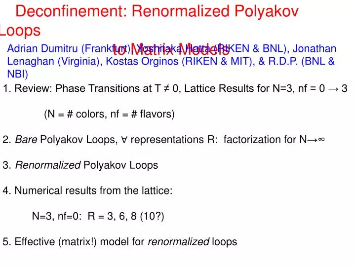
Deconfinement: Renormalized Polyakov Loops to Matrix Models Adrian Dumitru (Frankfurt), Yoshitaka Hatta (RIKEN & BNL), Jonathan Lenaghan (Virginia), Kostas Orginos (RIKEN & MIT), & R.D.P. (BNL & NBI) 1. Review: Phase Transitions at T ≠ 0, Lattice Results for N=3, nf = 0 → 3 (N = # colors, nf = # flavors) 2. Bare Polyakov Loops, ∀ representations R: factorization for N→∞ 3. Renormalized Polyakov Loops 4. Numerical results from the lattice: N=3, nf=0: R = 3, 6, 8 (10?) 5. Effective (matrix!) model for renormalized loops
Review of Lattice Results: N=3, nf = 0, 2, 2+1, 3 nf = 0: T_deconf ≈ 270 MeV pressure small for T < T_d like N→∞: p ~ 1 for T<T_d, p ~ N^2 for T>T_d (Thorn, 81) pressure/T^4 ↑ Bielefeld T=> nf ≠ 0: as nf ↑, p_ideal ↑, T_chiral ↓ BIG change: between nf = 0 and nf = 3, p_ideal: 16 to 48.5 x ideal m=0 boson Tc: 270 to 175 MeV! Even the order changes: first for nf=0 to “crossover” for nf = 2+1
Three colors, pure gauge: weakly first order Latent heat: ~ 1/3 vs 4/3 in bag model. So? Look at gauge-inv. correlation functions: (2-pt fnc. Polyakov loop) T < T_d : m = σ/T T > T_d: m = m_Debye T-dep. string tension ↑ ↑Debye mass Bielefeld .9 T_d ↑ T_d ↑ ↑ T_d ↑ 4 T_d (Some) correlation lengths grow by ~ 10!
Deconfining Transition vs N: First order ∀ N ≥ 4 Lucini, Teper, Wenger ‘03: latent heat ~ N^2 for N= 3, 4, 6, 8 N=2: second order => no latent heat N=3: “weakly” 1st N ≥ 4: strongly first order. x latent heat/N^2 x x 2 3 4 6 N=> Is N →∞ Gross-Witten? No data for Gross-Witten - First order but:
Flavor Independence Bielefeld Perhaps: even for nf ≠ 0, “transition” dominated by gluons At T ≠ 0: thermodynamics dominated by Polyakov loops
Wilson Lines at T ≠ 0 Always: “pure” SU(N) gauge, no dynamical quarks (nf = 0) Imaginary time formalism: Wilson line in fundamental representation: = propagator for “test quark”at x, moving up in (imaginary) time = propagator “test anti-quark” at x, moving back in time (Mandelstam’s constraint)
Polyakov Loops Wrap all the way around in τ: Polyakov loop = normalized loop = gauge invariant Confinement: test quarks don’t propagate Deconfinement: test quarks propagate Spontaneous breaking of global Z(N) = center SU(N) ‘t Hooft ‘79, Svetitsky and Yaffe, ‘82
Adjoint Representation Adjoint rep. = “test meson” Note: both coefficients ~ 1 Check: = dimension of the rep. Adjoint loop: divide by dim. of rep. At large N, = factorization
Two-index representations 2-index rep.’s = “di-test quarks” = symmetric or anti-sym. Di-quarks: two qks wrap once in time, or one qk wraps twice Again: both coeff’s ~ 1. Subscript = dimension of rep.’s = (N^2 ± N)/2 For arbitrary rep. R, if d_R = dimension of R, For 2-index rep.’s ±, as N →∞, corr.’s 1/N, not 1/N^2:
Loops at Infinite N “Conjugate” rep.’s of Gross & Taylor ‘93: If all test qks and test anti-qks wrap once and only once in time, Many other terms: dimension R = As N → ∞, if #, #’... are all of order 1, first term dominates, and: Normalization: if
Factorization at Infinite N In the deconfined phase, the fundamental loop condenses: Makeenko & Migdal ‘80: at N=∞, expectation values factorize: Phase trivial: = Z(N) charge of R, defined modulo N Magnitude not trivial: highest powers of win. At infinite N, any loop order parameter for deconfinement: even if e_R = 0! E.g.: adjoint loop (Damgaard, ‘87 ) vs adjoint screening. N.B.:
“Mass” renormalization for loops Loop = propagator for infinitely massive test quark. Still has mass renormalization, proportional to length of loop: a = lattice spacing. m_R = 0 with dimensional regularization, but so what? To 1-loop order in 3+1 dimensions: Divergences order by order in g^2. Only power law divergence for straight loops in 3+1 dim.’s. ; corrections ~aT. In 3+1 dim.’s, loops with cusps do have logarithmic divergence. (Dokshitzer: ~ classical bremstrahlung) In 2+1 dim.’s, straight loops also have log. div.’s. (cusps do not)
Renormalization of Wilson Lines Gervais and Neveu ‘80; Polyakov ‘80; Dotsenko & Vergeles ‘80 .... For irreducible representations R, renormalized Wilson line: = renormalization constant for Wilson line As R’s irreducible, different rep’s don’t mix under renormalization For straight lines in 3+1 dimensions, only: Noanomalous dim. for Wilson line: no condition to fix at some scale For all local, composite operators, Z’s independent of T Wilson line = non-local composite operator: temperature dependent: from 1/T, and (found numerically) Not really different: a m_R = func. renormalized g^2, and so T-dependent.
Renormalization of Polyakov Loops Renormalized loop: Constraint for bare loop: For renormalized loop: as a → 0, no constraint on ren.’d loop If E.g.: as T →∞, ren’d loops approach 1 from above: (Gava & Jengo ‘81) => negative “free energy” for loop Smooth large N limit:
Why all representations? Previously: concentrated on loops in fund. and adj. rep.’s, esp. with cusps. At T ≠ 0, natural for loops, at a given point in space, to wrap around in τ many times. Most general gauge invariant term: By group theory (the character expansion): Only this expression, which is linear in the bare loops, can be consistently ren.’d Note: If all Z_R => 0 as a=> 0, Irrelevant: physics is in the ren.’d, not the bare, loops. Discovered num.’y:
Lattice Regularization of Polyakov Loops Basic idea: compare two lattices. Same temperature, different lattice spacing If a << 1/T, ren’d quantities the same. N_t = # time steps = 1/(aT) changes between the two lattices: get Z_R N_s = # spatial steps; keep N_t/N_s fixed to minimize finite volume effects Numerically, Each f_R is computed at fixed T. As such, there is nothing to adjust. N.B.: also finite volume corrections from “zero” modes; to be computed. Explicit exp. of divergences to ~g^4 at a≠0: Curci, Menotti, & Paffuti, ‘85
Representations, N=3 Label rep.’s by their dimension: fundamental = adjoint = 8 symmetric 2-index = 6 special to N=3: anti-symmetric 2-index = “test baryon” = 10: Measured 3, 6, 8, & 10 on lattice
Lattice Results Standard Wilson action, three colors, quenched. Lattice coupling constant = coupling for deconfining transition: Non-perturbative renormalization: To get the same T/T_d @ different N_t, must compute at different Calculate grid in β, interpolate to get the same T/T_d at different N_t N.B. : Method same with dynamical quarks Measured (No signal for 10 for N_t > 4)
Bare triplet loop vs T, at different Nt Note scale=> ~ .3 Nt=4 Nt = # time steps. Bare loop vanishes as Nt →∞ Nt=6 Triplet loop↑ Nt=8 Nt=10 Tc T/Tc=>
Bare sextet loop vs T, at different Nt Note scale=> ~ .04 Nt = # time steps. Bare loop vanishes more quickly as Nt →∞ Nt=4 Sextet loop↑ Nt=6 Nt=8 Nt=10 Tc T/Tc=>
Bare octet loop vs T, at different Nt Note scale=> ~ .06 Nt=4 Very similar to sextet loop Octet loop↑ Nt=6 Nt=8 Nt=10 Tc T/Tc=>
Bare decuplet loop vs T, at different Nt Note scale=> ~ .006 Nt=4 No stat.’y significant signal for decuplet loop above Nt=4. Decuplet loop↑ Nt=6 Nt=8 Nt=10 Tc T/Tc=>
a m_R looks like usual “mass”: smooth function of ren.’d g^2 =>smooth func. of T: except near T_d!One loop: m_R ~ C_R; OK for T ~ 3 T_d. Fails for T < 1.5 T_d Casimir scaling for: a m_R ↓ a m_R ↑ T_d ↑ T/T_d =>
Renormalized Polyakov Loops Find: ren.’d triplet loop, but also significant octet and sextet loops, as well. Ren’d loop ↑ T_d ↑ T/T_d => No signal of decuplet loop at N_t > 4; C_10 big, so bare loop small
Results for Ren’d Polyakov Loops Like large N: Greensite & Halpern ‘81, Damgaard ‘87... (Similar to measuring adjoint string tension in confined phase) Transition first order →ren.’d loops jump at T_d: T > T_d: Find ordering: 3 > 8 > 6. But compute difference loops:
Difference Loops: Test of Factorization at N=3 Details of spikes near T_d? Sharp octet spike Broad sextet spike <= 8 <= 6 Max. octet diff. loop => Max. sextet diff. loop => T_d ↑
Bare Loops don’t exhibit Factorization Bare octet difference loop/bare octet loop: violations of factor. 50% @ Nt =4 200% @ Nt = 10.
Bielefeld’s Renormalized Polyakov Loop Kaczmarek, Karsch, Petreczky, & Zantow ‘02 Approx. agreement. Need 2-pt fnc at one N_t vs 1-pt fnc at several N_t
Bielefeld’s Ren’d Polyakov Loop, N=2 Digal, Fortunato, & Petreczky ‘02 Transition second order:
Mean Field Theory for Fundamental Loop At large N, if fundamental loop condenses, factorization ⇒ all other loops This is a mean field type relation; implies mean field for General effective lagrangian for renormalized loops: Choose basic variables as Wilson lines, not Polykov loops: (i = lattice sites) Loops automatically have correct Z(N) charge, and satisfy factorization. Effective action Z(N) symmetric. Potential terms (starts with adjoint loop): and next to nearest neighbor couplings: In mean field approximation, that’s it. (By using character exp.)
Matrix Model (=Mean Field) for N=3 Simplest possible model: only (Damgaard, ‘87) to get Fit Find linear in T Now compute loops in other representations using this
N=3: Lattice Results vs Simple Mean Field 3=> Solid lines = matrix model. Points = lattice data for renormalized loops. 8=> <= 6 <=10 ? Approximate agreement for 6 & 8. Predicts signal for 10!
Difference Loops for Matrix Model, N=3 <= Octet diff. loop Curves = difference loops computed in matrix model Large N => octet diff. loop < sextet diff. loop Max. ~ - .03 matrix model => vs -0.20 lattice Sextet diff. loop => Max. ~ - .07 matrix model => vs -0.25 lattice T_d ↑ 4 T_d ↑ Diff. loops: matrix model much broader & smaller than lattice data! => new physics in lattice.
Matrix Model, N=∞, and Gross-Witten Consider mean field, where the only coupling is Gross & Witten ‘80, Kogut, Snow, & Stone ‘82, Green & Karsch ‘84 At N=∞, mean field potential is non-analytic, given by two different potentials: For fixed β, the potential is everywhere continuous, but its third derivative is not, at the point = confined phase = deconfined phase
Gross-Witten Transition: “Critical” First Order Transition first order. Order parameter jumps: 0 to 1/2. Also, latent heat ≠ 0: But masses vanish, asymmetrically, at the transition! If β∼T, and the deconfining transition is Gross-Witten at N=∞, then the string tension and the Debye mass vanish at T_d as: But what about higher terms in the “potential”?
String related analysis @ large N hep-th/0310285: Aharony, Marsano, Minwalla, Papadodimas, Van Raamsdonk hep-th/0310286: Furuuchi, Schridber, & Semenoff By integrating over vev, one can show model with mean field same as model with just adjoint loop in potential. => Most general potential @ large N: Gross-Witten simplest model: c2 ≠ 0, c4=c6=...=0. AMMPR: consider c4 ≠ 0. Work in small volume, => compute at small g^2. AMMPR: either: 2nd order, or 1st order, Lattice for N=3: close to infinite N, with small c4, c6....? => close to Gross-Witten?
To do Two colors: matching critical region near T_d to mean field region about T_d? Higher rep.’s, factorization at N=2? Three colors: better measurements, esp. near T_d: “Spikes” in sextet and octet loops? Fit to matrix model? For decuplet loop, use “improved” Wilson line? HTL’s Four colors: is transition Gross-Witten? Or is N=3 an accident? With dynamical quarks: method to determine ren.’d loop(s) identical
Bielefeld: Ren’d loop with quarks. ≈ Same! Kaczmarek et al: hep-lat/0312015 c/o quarks Ren’d triplet loop ↑ c quarks Tc T/Tc=>