Download

1 / 54
590 likes | 1.21k Views
Capital Asset Pricing and Arbitrage Pricing Theory. 7. Bodie, Kane, and Marcus Essentials of Investments, 9 th Edition. 7.1 The Capital Asset Pricing Model. 7.1 The Capital Asset Pricing Model. Assumptions Markets are competitive, equally profitable

E N D
Capital Asset Pricing and Arbitrage Pricing Theory 7 Bodie, Kane, and Marcus Essentials of Investments, 9th Edition
7.1 The Capital Asset Pricing Model • Assumptions • Markets are competitive, equally profitable • No investor is wealthy enough to individually affect prices • All information publicly available; all securities public • No taxes on returns, no transaction costs • Unlimited borrowing/lending at risk-free rate • Investors are alike except for initial wealth, risk aversion • Investors plan for single-period horizon; they are rational, mean-variance optimizers • Use same inputs, consider identical portfolio opportunity sets
7.1 The Capital Asset Pricing Model • Hypothetical Equilibrium • All investors choose to hold market portfolio • Market portfolio is on efficient frontier, optimal risky portfolio
7.1 The Capital Asset Pricing Model • Hypothetical Equilibrium • Risk premium on market portfolio is proportional to variance of market portfolio and investor’s risk aversion • Risk premium on individual assets • Proportional to risk premium on market portfolio • Proportional to beta coefficient of security on market portfolio
7.1 The Capital Asset Pricing Model • Passive Strategy is Efficient • Mutual fund theorem: All investors desire same portfolio of risky assets, can be satisfied by single mutual fund composed of that portfolio • If passive strategy is costless and efficient, why follow active strategy? • If no one does security analysis, what brings about efficiency of market portfolio?
7.1 The Capital Asset Pricing Model • Risk Premium of Market Portfolio • Demand drives prices, lowers expected rate of return/risk premiums • When premiums fall, investors move funds into risk-free asset • Equilibrium risk premium of market portfolio proportional to • Risk of market • Risk aversion of average investor
7.1 The Capital Asset Pricing Model • The Security Market Line (SML) • Represents expected return-beta relationship of CAPM • Graphs individual asset risk premiums as function of asset risk • Alpha • Abnormal rate of return on security in excess of that predicted by equilibrium model (CAPM)
7.1 The Capital Asset Pricing Model • Applications of CAPM • Use SML as benchmark for fair return on risky asset • SML provides “hurdle rate” for internal projects
Figure 7.4 Scatter Diagram/SCL: Google vs. S&P 500, 01/06-12/10
7.2 CAPM and Index Models • Estimation results • Security Characteristic Line (SCL) • Plot of security’s expected excess return over risk-free rate as function of excess return on market • Required rate = Risk-free rate + β x Expected excess return of index
7.2 CAPM and Index Models • Predicting Betas • Mean reversion • Betas move towards mean over time • To predict future betas, adjust estimates from historical data to account for regression towards 1.0
7.3 CAPM and the Real World • CAPM is false based on validity of its assumptions • Useful predictor of expected returns • Untestable as a theory • Principles still valid • Investors should diversify • Systematic risk is the risk that matters • Well-diversified risky portfolio can be suitable for wide range of investors
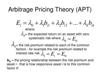
7.5 Arbitrage Pricing Theory • Arbitrage • Relative mispricing creates riskless profit • Arbitrage Pricing Theory (APT) • Risk-return relationships from no-arbitrage considerations in large capital markets • Well-diversified portfolio • Nonsystematic risk is negligible • Arbitrage portfolio • Positive return, zero-net-investment, risk-free portfolio
7.5 Arbitrage Pricing Theory • Calculating APT • Returns on well-diversified portfolio
Table 7.5 Portfolio Conversion Steps to convert a well-diversified portfolio into an arbitrage portfolio *When alpha is negative, you would reverse the signs of each portfolio weight to achieve a portfolio A with positive alpha and no net investment.
Table 7.6 Largest Capitalization Stocks in S&P 500 Stock Weight Stock Weight
Table 7.7 Regression Statistics of S&P 500 Portfolio on Benchmark Portfolio, 01/06-12/10
7.5 Arbitrage Pricing Theory • Multifactor Generalization of APT and CAPM • Factor portfolio • Well-diversified portfolio constructed to have beta of 1.0 on one factor and beta of zero on any other factor • Two-Factor Model for APT
Table 7.9 Constructing an Arbitrage Portfolio Constructing an arbitrage portfolio with two systemic factors
Selected Problems 7-36
Problem 1 CAPM: E(ri) = rf + β(E(rM)-rf) a. CAPM: E(ri) = 5% + β(14% -5%) • E(rX) = • X = • E(rY) = • Y = 5% + 0.8(14% – 5%) = 12.2% 14% – 12.2% = 1.8% 5% + 1.5(14% – 5%) = 18.5% 17% – 18.5% = –1.5% 7-37
Problem 1 Which stock? Well diversified:Relevant Risk Measure?Best Choice? X = 1.8% Y = -1.5% • Which stock? • Held alone:Relevant Risk Measure?Best Choice? β: CAPM Model Calculate Sharpe ratios Stock X with the positive alpha 7-38
Problem 1 (continued) Sharpe Ratios Held Alone: (0.14 – 0.05)/0.36 = 0.25 (0.17 – 0.05)/0.25 = 0.48 Sharpe Ratio X = Sharpe Ratio Y = Sharpe Ratio Index = Better (0.14 – 0.05)/0.15 = 0.60 7-39
Problem 2 E(rP) = rf + b[E(rM) – rf] 20% = 5% + b(15% – 5%) b = 15/10 = 1.5 7-40
Problem 3 E(rP) = rf + b[E(rM) – rf] E(rp) when double the beta: If the stock pays a constant dividend in perpetuity, then we know from the original data that the dividend (D) must satisfy the equation for a perpetuity: Price = Dividend / E(r) $40 = Dividend / 0.13 At the new discount rate of 19%, the stock would be worth: $5.20 / 0.19 = $27.37 β = 0.75 13% = 7% + β(8%) or E(rP) = 7% + 1.5(8%) or E(rP) = 19% so the Dividend = $40 x 0.13 = $5.20 7-41
Problem 4 • False. b = 0 implies E(r) = rf , not zero. • Depends on what one means by ‘volatility.’ If one means the then this statement is false. Investors require a risk premium for bearing systematic (i.e., market or undiversifiable) risk. • False. You should invest 0.75 of your portfolio in the market portfolio, which has β= 1,and the remainder in T-bills. Then: • bP= (0.75 x 1) + (0.25 x 0) = 0.75 7-42
Problems 5 & 6 5. 6. Not possible. Portfolio A has a higher beta than Portfolio B, but the expected return for Portfolio A is lower. Possible. Portfolio A's lower expected rate of return can be paired with a higher standard deviation, as long as Portfolio A's beta is lower than that of Portfolio B. 7-43
Problem 7 7. Calculate Sharpe ratios for both portfolios: Not possible. The reward-to-variability ratio for Portfolio A is better than that of the market, which is not possible according to the CAPM, since the CAPM predicts that the market portfolio is the portfolio with the highest return per unit of risk. 7-44
Problem 8 8. Need to calculate Sharpe ratios? Not possible. Portfolio A clearly dominates the market portfolio. It has a lower standard deviation with a higher expected return. 7-45
Problem 9 9. Given the data, the SML is: E(r) = 10% + b(18% – 10%) A portfolio with beta of 1.5 should have an expected return of: E(r) = 10% + 1.5(18% – 10%) = 22% Not Possible: The expected return for Portfolio A is 16% so that Portfolio A plots below the SML (i.e., has an = –6%), and hence is an overpriced portfolio. This is inconsistent with the CAPM. 7-46
Problem 10 10. E(r) = 10% + b(18% – 10%) The SML is the same as in the prior problem. Here, the required expected return for Portfolio A is: 10% + (0.9 8%) = 17.2% Not Possible: The required return is higher than 16%. Portfolio A is overpriced, with = –1.2%. 7-47
Problem 11 11. Sharpe A = Sharpe M = Possible: Portfolio A's ratio of risk premium to standard deviation is less attractive than the market's. This situation is consistent with the CAPM. The market portfolio should provide the highest reward-to-variability ratio. (16% - 10%) / 22% = .27 (18% - 10%) / 24% = .33 7-48
Problem 12 12 Since the stock's beta is equal to 1.0, its expected rate of return should be equal to ______________________. E(r) = 0.18 = the market return, or 18% or P1 = $109 7-49
Problem 13 r1 = 19%; r2 = 16%; b1 = 1.5; b2 = 1.0 We can’t tell which adviser did the better job selecting stocks because we can’t calculate either the alpha or the return per unit of risk. CAPM: ri = 6% + β(14%-6%) r1 = 19%; r2 = 16%; b1 = 1.5; b2 = 1.0, rf = 6%; rM = 14% a1 = a2 = The second adviser did the better job selecting stocks (bigger + alpha) [6% + 1.5(14% – 6%)] = 19% – 18% = 1% 19% – 16% – 16% – 14% = 2% [6% + 1.0(14% – 6%)] = Part c? 7-50