P MODE TRAVEL TIME IN ACTIVE REGIONS USING TIME-DISTANCE METHOD

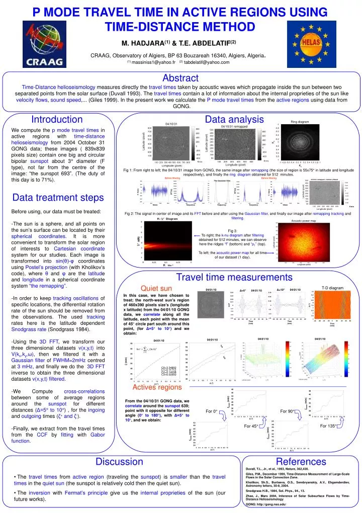
1. Abstract Introduction Travel time measurements Data analysis Ring diagram 04/10/31 -1 04/10/31 remapped 800 -0.8 800 500 -0.6 700 800 450 600 -0.4 600 400 600 400 350 -0.2 500 400 Latitude (pixel) Ky 200 300 0 Latitude (pixel) 400 200 250 0.2 0 0 300 200 0.4 -200 150 200 -200 0.6 100 -400 100 -400 0.8 50 -600 1 Km/s Km/s 100 200 300 400 500 600 100 200 300 400 500 600 700 800 -1 -0.8 -0.6 -0.4 -0.2 0 0.2 0.4 0.6 0.8 1 Longitude (pixel) Kx Longitude (pixel) 04/10/31 remapped + tracked +filtered 500 TheGaussian filtre 300 18000 1 14000 200 0.06 450 0.9 16000 200 12000 150 400 0.04 0.8 14000 10000 100 100 0.7 350 0.02 12000 0.6 8000 50 300 0 FFT(V) 0 Latitude (pixel) 10000 FFT(V) V Km/s V Km/s 0.5 0 -100 6000 250 -0.02 8000 0.4 -50 6000 200 -0.04 -200 0.3 4000 -100 4000 0.2 150 -300 -0.06 2000 -150 2000 0.1 100 -200 -400 0 0 0 -0.08 0 500 1000 1500 0 500 1000 1500 0 . 500 1000 1500 0 500 1000 1500 0 500 1000 1500 50 times frequency frequency frequency times 100 200 300 400 500 600 Km/s Longitude (pixel) Acousticpowermap T-D diagram 04/01/10 Δ=10° 04/01/10 Δ=5° 04/01/10 10 0.04 0.06 9.5 0.03 0.04 9 0.02 8.5 0.02 0.01 8 Δ (°) CCF 0 0 7.5 7 -0.01 -0.02 6.5 -0.02 6 -0.04 -0.03 5.5 -0.04 -0.04 -0.06 -80 -60 -40 -20 0 20 40 60 80 -80 -60 -40 -20 0 20 40 60 80 5 -80 -60 -40 -20 0 20 40 60 80 Time (min) Time (min) Time (min) 04/01/10 04/01/10 04/01/10 04/01/10 58 58 tp 56 56 54 54 52 tg 52 50 ζ (min) 48 50 46 48 C0=3.34892 C1=0.11712 C2=0.14038 C3=0.02650 44 46 42 44 40 5 5.5 6 6.5 7 7.5 8 8.5 9 9.5 10 5 5.5 6 6.5 7 7.5 8 8.5 9 9.5 10 Δ (°) Δ (°) 48 48 46 46 44 42 44 ζmean (min) 40 ζmean (min) 42 38 40 36 34 38 32 36 5 5.5 6 6.5 7 7.5 8 8.5 9 9.5 10 5 5.5 6 6.5 7 7.5 8 8.5 9 9.5 10 Δ (°) Δ (°) 50 50 48 48 46 46 44 44 ζmean (min) ζmean (min) 42 42 40 40 38 38 36 36 34 34 5 5.5 6 6.5 7 7.5 8 8.5 9 9.5 10 5 5.5 6 6.5 7 7.5 8 8.5 9 9.5 10 Δ (°) Δ (°) References Discussion M. HADJARA(1) & T.E. ABDELATIF(2) CRAAG, Observatory of Algiers, BP 63 Bouzareah 16340, Algiers, Algeria. (1) massiniss1@yahoo.fr (2) tabdelatif@yahoo.com Time-Distance helioseismology measures directly the travel times taken by acoustic waves which propagate inside the sun between two separated points from the solar surface (Duvall 1993). The travel times contain a lot of information about the internal proprieties of the sun like velocity flows, sound speed,... (Giles 1999). In the present work we calculate the P mode travel times from the active regions using data from GONG. P MODE TRAVEL TIME IN ACTIVE REGIONS USING TIME-DISTANCE METHOD We compute the p mode travel times in active regions with time-distance helioseismology from 2004 October 31 GONG data; these images ( 839x839 pixels size) contain one big and circular bipolar sunspot about 3° diameter (F type), not far from the centre of the image: “the sunspot 693”. (The duty of this day is to 71%). Data treatmentsteps Before using, our data must be treated: -The sun is a sphere, and all points on the sun’s surface can be located by their spherical coordinates. It is more convenient to transform the solar region of interests to Cartesian coordinate system for our studies. Each image is transformed into sin(θ)-φ coordinates using Postel’s projection (with Kholikov’s code), where θ and φ are the latitude and longitude in a spherical coordinate system “the remapping”. -In order to keep tracking oscillations of specific locations, the differential rotation rate of the sun should be removed from the observations. The used tracking rates here is the latitude dependent Snodgrass rate (Snodgrass 1984). -Using the 3D FFT, we transform our three dimensional datasets v(x,y,t) into V(kx,ky,ω), then we filtered it with a Gaussian filter of FWHM=2mHz centred at 3 mHz, and finally we do the 3D FFT inverse to obtain the three dimensional datasets v(x,y,t) filtered. -We Compute cross-correlations between some of average regions around the sunspot for different distances (Δ=5° to 10°) , for the ingoing and outgoing times (ζ+ and ζ-). -Finally, we extract from the travel times from the CCF by fitting with Gabor function. Longitude (pixel) Fig 1: From right to left; the 04/10/31 image from GONG, the same image after remapping (the size of region is 55x75° in latitude and longitude respectively), and finally the ring diagram obtained for 512 minutes. Beforefiltering Beforefiltering Fig 2: The signal in center of image and its FFT before and after using the Gaussian filter, and finally our image after remapping tracking and filtering. Fig 3: To right; the k-nu diagram after filtering obtained for 512 minutes, we can observe here the ridges “f” (bottom) and “p1” (top). To left; the acoustic power map for all time of our dataset (1 day). Quietsun In this case, we have chosen to treat; the north-west sun’s region of 460x390 pixels size’s (longitude x latitude) from the 04/01/10 GONG data, we correlate along all the latitude, each point with the mean of 45° circle part south around this point, (for Δ=5° to 10°) and we obtain: -0.04 80 Actives regions From the 04/10/31 GONG data, we correlate around the sunspot 639; point with it opposite for different angle (0° to 180°), with Δ=5° to 10°, and we obtain: For 0° For 90° For 135° For 45° Duvall, T.L., Jr., et al., 1993, Nature, 362,430. Giles, P.M., December 1999, Time-Distance Measurement of Large-Scale Flows in the Solar Convection Zone. Kholikov, Sh.S., Burtseva, O.S., Serebryanskiy, A.V., Ehgamderdiev, Astronomy letters, 30-8, 2004. Snodgrass H.B., 1984, Sol. Phys., 94., 13. Zhao, J., Mars 2004, Inference of Solar Subsurface Flows by Time-Distance Helioseismology GONG: http://gong.nso.edu/ • The travel times from active region (traveling the sunspot) is smaller than the travel times in the quiet sun (the sunspot is relatively cold then the quiet sun). • The inversion with Fermat’s principle give us the internal proprieties of the sun (our future works).