Download

1 / 17
170 likes | 193 Views
7. Stability. 7.1 System stability. [Ref:Rao]. DEU-MEE 5017 Advanced Automatic Control. [Ref: Rao]: Continue. Different Types of Stability:. Locations ofcharacteristic roots (.) and the corresponding responses :. A fundemental definition of system stability :. Example 7.1 :.

E N D
7. Stability 7.1 Systemstability [Ref:Rao] DEU-MEE 5017 Advanced Automatic Control
Locations ofcharacteristic roots (.) and the corresponding responses :
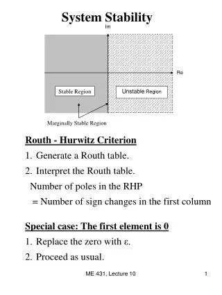
Example 7.2 : Study the system stability by Routh-Hurwitz method.
7.2.1Special case-1: (The first element in a row is zero) For this case, the first element in a row is zero, with at least one nonzero element in the same row. This problem can be solved by replacing the first element of the row, which is zero, with a small number , which can be assumed to be either positive or negative. The array is completed as mentioned before. The number of roots of the polynomial in RHP is then equal to the number of sign changes in the first column. Example :
7.2.2Special case-2: (The elements in a onerowareallzero) • The auxilary equation A(s) is used. A(s) is formed from the coefficients of the above the row of zeros in the Routh array. The roots of A(s) also satisfy the original equation. • Take the derivative of A(s) with respect to s; this gives dA(s)/ds=0. Replace the row of zeros with the coefficients of dA(s)/ds=0. • Replace the row of zeros with the coefficients of dA(s)/ds=0. • Continue with Routh array in the usual manner and interpret the change of signs. Example :
R ( s ) Example 7.3 : Find the range of K so that the closed loop system is stable. D(s)= Rule-1: Coefficients in the characteristic equation must have same signs. Routh array: Rule-2: Resulting coefficients in the first column of the Routh array must have same signs. So, the range of K for the stable system:
7.3 Ziegler-Nichols Design In practice, the coefficients of a control system should be set so that the closed –loop system has an optimum response. Depending on the controller type, the critical gain, the integral time constant,and the derivative time constant can be determined based on experimental and computational methods. One of these method is the Ziegler-Nichols method. Ziegler-Nichols Design: 1.Use step input for the reference. 2.Start controlling the system with a constant gain, K. 3.Increase K so that the closed-loop response has a continuous oscillation response. 4. In case of the continous oscillation response, choose the control gain and measure the period of the response. Then , design the control system. Kc: Critical gain. Tc: Oscillation period.
R ( s ) Example 7.4: Consider Example 7.3. Design the control system (P, PI, PID.) by the Ziegler-Nichols method. D(s)= Critical gain: (Determined from the Routh-Hurwitz method) MATLAB: >> a=[1,6,11,6,10];roots(a)
Pcontrol: PI control: PID control:
Study and compare the closed-loop responses of P, PI and PID control.