Download
1 / 33
330 likes | 338 Views
Explore topics in gravitational wave analysis from interferometers, including the cross-correlation statistic for identifying co-incident bursts. Learn about LIGO, types of gravitational waves, LISA, and more.

E N D
Topics in Data Analysis from Gravitational Wave Interferometers, including a Cross Correlation Statistic to Identify Co-incident bursts • Brief Introduction to LIGO • What is a Gravitational Wave? • Primary Types of GWs • Gravitational Wave Interferometers • LIGO and its sister projects • LISA • GW Bursts • Cross Correlation Statistic to Identify Co-incident Bursts • Simulation of Time Delay Interferometry in LISA Surjeet Rajendran, Caltech
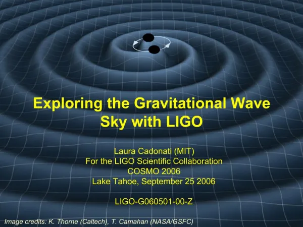
Gravitational Waves • Static Gravitational fields are described in General Relativity as a curvature or warpage of space-time, changing the distance between space-time events • Special Relativity requires that “news” about changes in the gravitational field cannot travel faster than the velocity of light (‘c’) • The “news” about the changing gravitational field propagates outward as gravitational radiation – a wave of spacetime curvature. • When a plane polarized Gravitational Wave passes through space, it stretches and squeezes space along mutually perpendicular axes which form a plane orthogonal to the direction of propagation of the GW. • These strecthes and squeezes can be expressed as a strain in space . • Plane polarized Gravitational Waves come in 2 polarizations: the “+” Polarization and the “x” polarization. Surjeet Rajendran, Caltech
Types of extra-terrestrial GW emissions • Bursts • Collapse of a star into a Neutron star or Black Hole • Fall of stars and small black holes into super massive black holes • Asymmetric supernova explosions • Chirps • Coalescence of compact binaries • Periodic Waves • Rotating Neutron and Binary Star systems • Stochastic Waves • Primarily from the Big Bang Surjeet Rajendran, Caltech
Gravitational Wave Interferometers Surjeet Rajendran, Caltech
LIGO and its sister projects Surjeet Rajendran, Caltech
Laser Interferometer Space Antenna (LISA) • Constellation of 3 spacecraft • Able to search for low frequency gravitational waves owing to lack of seismic noise • Primarily searches for low frequency periodic waves from compact binaries, neutron stars and black holes Surjeet Rajendran, Caltech
GW Bursts • The waveform of a GW Burst depends primarily on the dynamics of the source and therefore, burst waveform templates are difficult to create and hence Matched filtering techniques can’t be reliably employed. • Classical Methodology adopted to detect Bursts by LDAS (LIGO Data Analysis System): • LDAS contains algorithms like Slope, tfClusters and Power (also called DSOs or Event Trigger Generators) which identify peaks of excess power in sensitive frequency bands of the data-stream • Upon identification, the algorithms fill up a meta-database with such candidate burst triggers • Each burst trigger contains information about the central frequency, amplitude, start-time and duration of the corresponding burst. • To identify co-incident bursts, we require the candidate burst triggers to have similar central frequencies, amplitude, duration and appropriately delayed start-times (which is 10 ms for the 2 LIGO observatories at Hanford and Livingston) Surjeet Rajendran, Caltech
Cross-correlation of coincident burst data • After the search DSOs have identified data segments in which a burst is apparently present, • And processing of the triggers identifies H2/L1 pairs which are coincident in time (to the level of resolution of the DSOs, eg, 1/8 second for tfclusters, ie, not as good as the required 10 msec), • And trigger level consistency cuts are made (overlapping frequency band, consistent amplitudes, etc) • We still may have to reduce the coincident fake rate. • SO, go back to the raw data and require consistency: • We seek a statistical measure which • reduces false coincidences significantly while • maintaining very high efficiency for even the faintest injected burst which triggers the DSOs • And can provide a better estimate of the start-time coincidence • We require this statistic to be robust even when • the two IFOs have very different sensitivities as well as • when there is a time delay of +/- 10 ms between the injected signals in the two IFOs. Surjeet Rajendran, Caltech
Cross-correlation statistic Let: X(t) = DT seconds of data from H2 Y(t) = DT seconds of data from L1. CXY(f) = Coherence function between X, Y. = abs(CSD(X, Y)2)/(PSD(X)*PSD(Y)) (CSD = Cross Spectral Density, PSD = Power Spectral density) Consider the statistic: CCS = Integral (CXY, {fmin, fmax}) (or) since we are sampling the data at discrete time intervals, we use the following discrete analog of (*): CCS = S CXY(f)*Df (between fmin and fmax) In our analysis, we use the value of DT = 1 second. The statistic will depend upon the value of DT and this dependence needs to be explored. Surjeet Rajendran, Caltech
Evaluation of the CCS • The idea behind this exercise is to determine the distribution of the CCS statistic before and after signal injection • and thereby hope to find a value of the CCS statistic which can then be used as a test to identify coincident bursts. • We would like this statistic to have a high efficiency of detection while maintaining a low fake rate. Surjeet Rajendran, Caltech
Determination of optimal values of fmin and fmax • We are considering ZM waveforms at a distance of 2 parsec (limit of sensitivity during E7) • To find the optimal range of values of fmin and fmax, we plot CXY(f) for the case when there are no injected burst signals in H2, L1 and compare it with the case when we inject signals. Surjeet Rajendran, Caltech
CCS for different ZM waveforms Surjeet Rajendran, Caltech
Limits of integration • From the above plots, it is clear that the region of interest lies between ~250 Hz – 1000 Hz. • This is consistent with the fact that ZM supernovae have little power beyond 1000 Hz and the fact that LIGO has its peak sensitivity in this region. • The plots also indicate that the CCS statistic would be of little use in detecting some weak waveforms (eg: A1B1G5). • Details: • The raw E7 data has been whitened and resampled to 4096 Hz • The injected signals have been filtered through the calibrated transfer function (strain LSC-AS_Q counts), then whitened and resampled like the data. • So far, we have been using 300-1000 Hz as our limits of integration. Surjeet Rajendran, Caltech
Procedure for evaluating CCS • We take N (N = 360 in our case) seconds of data from L1 and H2. • We break the N second dataset into (N/DT) intervals of length DT each (DT= 1 second in our case). • We then estimate the distribution of the CCS statistic on the raw data by forming (N/ DT)2 coincidences between them and computing the CCS statistic between the DT second intervals thus generated. • We histogram the results to arrive at the distribution of the CCS statistic on the raw data. • Since the CCS statistic test will be used only on the data sections that trigger the DSOs, we perform the same analysis on the data sections between the times t and t + DT where t corresponds to the time identified by the DSO as the start time of the burst which triggered the DSO. • We then inject ZM waveform signals in the (N/DT) intervals of length DT. • The distribution of the CCS statistic after signal injection is similarly studied. • We then inject the ZM waveform signals with a time delay of 10 ms (H2/L1 light travel time) between them and estimate the CCS statistic by the above method. Surjeet Rajendran, Caltech
Summary of results Surjeet Rajendran, Caltech
Observations • the distribution of the CCS statistic on the data sections identified by the DSOs as containing bursts is very similar to the distribution of the CCS statistic on random DT seconds of data from L1 and H2. • The peak of the CCS statistic distribution when the signal between H2, L1 is delayed by 10 ms is occurs at a slightly lower bin than the peak of the distribution when there is no delay. • However, we can still produce an efficient value of the CCS statistic which maintains high rates of efficiency while minimizing the fake rate. Surjeet Rajendran, Caltech
Cut on CCS. Efficiency vs fake rate reduction Surjeet Rajendran, Caltech
Some things to be done • Estimate the CCS between 250-1000 Hz. We expect the results to be better than the results obtained above (using 300-1000 Hz). • Explore the dependence of the CCS on DT. Can we estimate DT to 10 msec or better? • Explore other waveforms • S1 data • Automate, using LDAS (or DMT). Surjeet Rajendran, Caltech
Laser Frequency and Spacecraft motion noise in LISA • The dynamics of the LISA constellation is such that it is impossible to maintain equal arm lengths between LISA spacecraft. • Laser frequency fluctuations are therefore not cancelled. • The Nd:YAG Laser to be used in LISA offers a frequency stability of 10-13Hz1/2 • The GW sources for LISA cause fluctuations of the order of 10-20Hz1/2 • Similarly, random motions of the optical benches induce Doppler shifts (of similar order as the Laser Frequency Fluctuations). • These noise sources must therefore be cancelled up to at least second order for effective performance of the LISA constellation. Surjeet Rajendran, Caltech
The LISA System • Each vertex spacecraft contains two rigid optical benches (the benches are attached to each other by an optic fiber) shielding two (almost) inertial proof masses. • Each optical bench has its own laser, which is used to both exchange signals with one of the distant spacecraft and also to exchange signals with the adjacent optical bench. • Thus, there are six optical benches, six lasers, and a total of twelve Doppler time series observed. • An outgoing light beam transmitted to a distant spacecraft is routed from the laser on the local optical bench using mirrors and beam splitters; this beam does not interact with the local proof mass. • Conversely, an incoming light beam from a distant spacecraft is bounced off the local proof mass before being reflected onto the photo-detector where it is mixed with light from the laser on that same optical bench. • Beams between adjacent optical benches however do precisely the OPPOSITE. Surjeet Rajendran, Caltech
Notation • Y31 is the fractional (or normalized by center frequency) Doppler series derived from reception at spacecraft 1 with transmission from spacecraft 2. Similarly, Y21 is the Doppler time series derived from reception at spacecraft 1 with transmission at spacecraft 3. • We also use a useful notation for delayed data streams: Y31,23 = Y31 (t-L2 - L3) • Six more Doppler series result from Laser beams exchanged between adjacent optical benches; these are similarly indexed as Zij • The fractional frequency fluctuations of the laser on the optical bench on spacecraft 1 which exchanges signals with spacecraft 2 is labeled C1. • The random velocity of this optical bench is labeled V1 while the random velocity of the proof mass associated with this bench is labeled v1. • The shot noise contribution to the Doppler time series Yij is denoted by Yijshot , while the effect of a passing gravitational wave on the time series Yij is denoted by YijGW. Surjeet Rajendran, Caltech
Output at the Photodetectors • Y21 = C3,2 – n2. V3,2 + 2n2.v1* - n2.V1* - C1* + Y21GW + Y21shot • Z21 = C1 + 2n3.(v1 – V1) – C1* • Y31 = C2,3*+ n3. V2,3* - 2n3.v1 + n3.V1 - C1 + Y31GW + Y31shot • Z31 = C1* - 2n2.(v1* – V1*) – C1 Surjeet Rajendran, Caltech
Noise Cancelling Combinations • Work of Armstrong, Estabrook and Tinto (JPL) • By taking appropriate combinations of the Doppler time series, we can cancel the Laser Frequency Fluctuations and Spacecraft motion effects up to second order • In fact, complete cancellation of the Laser frequency noise is possible if we accurately knew the arm-lengths • Tinto, Estabrook and Armstrong’s analysis shows that these combinations are highly effective when the arm-lengths are known with realizable precision. • Examples: • X = Y32, 322 – Y23,233 + Y31,22 – Y21,33 + Y23,2 – Y32,3 + Y21 – Y31 + (1/2) * ( - Z21,2233 + Z21,33 + Z21,22 –Z21) + (1/2) * ( Z31,2233 – Z31,33 – Z31,22 + Z31) • a = Y21 – Y31 + Y13,2 – Y12,3 + Y32,12 – Y23,13 - (1/2) * (Z13,2 + Z13,13 + Z21 + Z21,123 + Z32,3 + Z32,12) + (1/2) * (Z23,2 + Z23,13 + Z31 + Z31,123 + Z12,3 + Z12,12) Surjeet Rajendran, Caltech
Details of the Simulation • Doppler data received at each spacecraft has been preprocessed • Distances between the spacecraft (L1, L2 and L3) are precisely known • The simulation therefore deals with a system which consists of three almost but not precisely stationary spacecraft (ie: each spacecraft is assumed to have a small random velocity), the spacecraft forming the vertices of a triangle with known sides. • The Doppler data represented in this simulation is normalized by central frequency (300 THz corresponding to 1 mm wavelength laser light from the Nd:YAG Lasers). • Noise spectra obtained from LISA Pre-Phase A report. • The data for the simulation was generated and sampled at 2 Hz since LISA is maximally sensitive between 10-4 Hz – 1 Hz. • Since we require a frequency resolution of at least 10-4 Hz, the simulation was executed to obtain a week (604800 seconds) of LISA data and the power spectrum of the gathered data in the combinations described above was then estimated. • The simulation in its current state accepts only elliptically polarized sinusoidal gravitational waves (LISA sensitivities have been traditionally given for sinusoidal waves). • Simulation created in Matlab Surjeet Rajendran, Caltech
Results Surjeet Rajendran, Caltech
Results Surjeet Rajendran, Caltech
Results Surjeet Rajendran, Caltech
Results Surjeet Rajendran, Caltech
Results Surjeet Rajendran, Caltech
Results Surjeet Rajendran, Caltech
Results Surjeet Rajendran, Caltech
Results Surjeet Rajendran, Caltech
Conclusions • The noise canceling combinations a and X successfully cancel the laser frequency fluctuation noise and spacecraft motion effects to acceptable levels while allowing us to detect the gravitational wave. • The noise spectra obtained from the simulation are identical to the spectra obtained by Armstrong, Estabrook and Tinto through an analytic calculation of the appropriate transfer functions. • Thus, the simulation quantitatively demonstrates that Time Delay Interferometry can be successfully implemented in LISA to recover the gravitational wave signal even when the system is swamped by laser frequency fluctuation noise and spacecraft motion effects. The gravitational wave sensitivity of LISA is then limited by acceleration noise (at low frequencies) and shot noise (at high frequencies). Surjeet Rajendran, Caltech