Download
1 / 48
500 likes | 592 Views
Pattern Classification All materials in these slides were taken from Pattern Classification (2nd ed) by R. O. Duda, P. E. Hart and D. G. Stork, John Wiley & Sons, 2000 with the permission of the authors and the publisher. Introduction Maximum-Likelihood Estimation

E N D
Pattern ClassificationAll materials in these slides were taken fromPattern Classification (2nd ed) by R. O. Duda, P. E. Hart and D. G. Stork, John Wiley & Sons, 2000 with the permission of the authors and the publisher
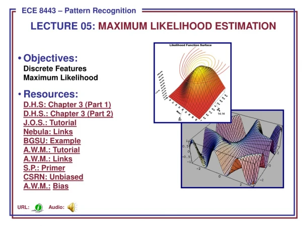
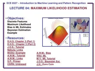
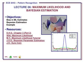
Introduction Maximum-Likelihood Estimation Example of a Specific Case The Gaussian Case: unknown and Bias Appendix: ML Problem Statement Chapter 3:Maximum-Likelihood & Bayesian Parameter Estimation (part 1)
Introduction • Data availability in a Bayesian framework • We could design an optimal classifier if we knew: • P(i) (priors) • P(x | i) (class-conditional densities) Unfortunately, we rarely have this complete information! • Design a classifier from a training sample • No problem with prior estimation • Samples are often too small for class-conditional estimation (large dimension of feature space!) Pattern Classification, Chapter 3 1
A priori information about the problem • Normality of P(x | i) P(x | i) ~ N( i, i) • Characterized by 2 parameters • Estimation techniques • Maximum-Likelihood (ML) and the Bayesian (Maximum A Posteriori-MAP) estimations • Results are nearly identical, but the approaches are different Pattern Classification, Chapter 3 1
Parameters in ML estimation are fixed but unknown! • Best parameters are obtained by maximizing the probability of obtaining the samples observed • Bayesian (MAP) methods view the parameters as random variables having some known distribution • In either approach, we use P(i | x)for our classification rule! Pattern Classification, Chapter 3 1
Maximum-Likelihood Estimation • Has good convergence properties as the sample size increases • Simpler than any other alternative techniques • General principle • Assume we have c classes and P(x | j) ~ N( j, j) P(x | j) P (x | j, j) where: Pattern Classification, Chapter 3 2
Use the informationprovided by the training samples to estimate = (1, 2, …, c), each i (i = 1, 2, …, c) is associated with each category • Suppose that D contains n samples, x1, x2,…, xn • ML estimate of is, by definition the value that maximizes P(D | ) “It is the value of that best agrees with the actually observed training sample” Pattern Classification, Chapter 3 2
Optimal estimation • Let = (1, 2, …, p)t and let be the gradient operator • We define l() as the log-likelihood function l() = ln P(D | ) • New problem statement: determine that maximizes the log-likelihood Pattern Classification, Chapter 3 2
Set of necessary conditions for an optimum is: l = 0 Pattern Classification, Chapter 3 2
Example of a specific case: unknown • P(xi | ) ~ N(, ) (Samples are drawn from a multivariate normal population) = , therefore: • The ML estimate for must satisfy: Pattern Classification, Chapter 3 2
Multiplying by and rearranging, we obtain: Just the arithmetic average of the samples of the training samples! Conclusion: If P(xk | j) (j = 1, 2, …, c) is supposed to be Gaussian in a d-dimensional feature space; then we can estimate the vector = (1, 2, …, c)t and perform an optimal classification! Pattern Classification, Chapter 3 2
ML Estimation: • Gaussian Case: unknown and = (1, 2) = (, 2) Pattern Classification, Chapter 3 2
Summation: Combining (1) and (2), one obtains the ML estimates: Pattern Classification, Chapter 3 2
Bias • ML estimate for 2 is biased • An elementary unbiased estimator for is: Pattern Classification, Chapter 3 2
Appendix: ML Problem Statement • Let D = {x1, x2, …, xn} P(x1,…, xn | ) = 1,nP(xk | ); |D| = n Our goal is to determine (value of that makes this sample the most representative!) Pattern Classification, Chapter 3 2
|D| = n . . . . x2 . . x1 xn N(j, j) = P(xj, 1) P(xj | 1) P(xj | k) D1 x11 . . . . x10 Dk . Dc x8 . . . x20 . . x1 x9 . . Pattern Classification, Chapter 3 2
= (1, 2, …, c) Problem: find such that: Pattern Classification, Chapter 3 2
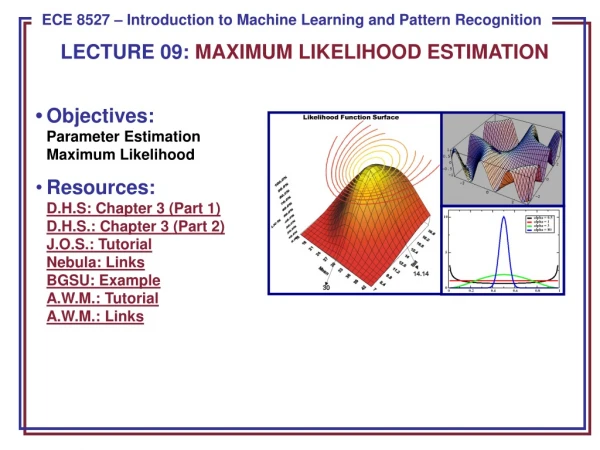
Chapter 3:Maximum-Likelihood and Bayesian Parameter Estimation (part 2) • Bayesian Estimation (BE) • Bayesian Parameter Estimation: Gaussian Case • Bayesian Parameter Estimation: General Estimation • Problems of Dimensionality • Computational Complexity • Component Analysis and Discriminants • Hidden Markov Models
Bayesian Estimation (Bayesian learning to pattern classification problems) • In MLE was supposed fixed • In BE is a random variable • The computation of Posterior probabilities P(i | x) lies at the heart of Bayesian classification • Goal: compute P(i | x, D) Given the sample D, Bayes formula can be written Pattern Classification, Chapter 3 3
To demonstrate the preceding equation, use: Pattern Classification, Chapter 3 3
Bayesian Parameter Estimation: Gaussian Case Goal: Estimate using the a-posteriori density P( | D) • The univariate case: P( | D) is the only unknown parameter (0 and 0 are known!) Pattern Classification, Chapter 3 4
Reproducing density Identifying (1) and (2) yields: Pattern Classification, Chapter 3 4
The univariate case P(x | D) • P( | D) computed • P(x | D) remains to be computed! It provides: (Desired class-conditional density P(x | Dj, j)) Therefore: P(x | Dj, j) together with P(j) And using Bayes formula, we obtain the Bayesian classification rule (Maximum A Posteriori) : Pattern Classification, Chapter 3 4
Bayesian Parameter Estimation: General Theory • P(x | D) computation can be applied to any situation in which the unknown density can be parametrized: the basic assumptions are: • The form of P(x | ) is assumed known, but the value of is not known exactly • Our knowledge about is assumed to be contained in a known prior density P() • The rest of our knowledge is contained in a set D of n random variables x1, x2, …, xn that follows P(x) Pattern Classification, Chapter 3 5
The basic problem is: “Compute the posterior density P( | D)” then “Derive P(x | D)” Using Bayes formula, we have: And by independence assumption: Pattern Classification, Chapter 3 5
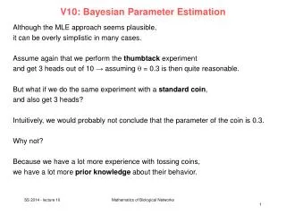
Problems of Dimensionality • Problems involving 50 or 100 features (binary valued) • Classification accuracy depends upon the dimensionality and the amount of training data • Case of two classes multivariate normal with the same covariance Pattern Classification, Chapter 3 7
If features are independent then: • Most useful features are the ones for which the difference between the means is large relative to the standard deviation • It has frequently been observed in practice that, beyond a certain point, the inclusion of additional features leads to worse rather than better performance: we have the wrong model ! Pattern Classification, Chapter 3 7
7 7 Pattern Classification, Chapter 3 7
Computational Complexity • Our design methodology is affected by the computational difficulty • “big oh” notation f(x) = O(h(x)) “big oh of h(x)” If: (An upper bound on f(x) grows no worse than h(x) for sufficiently large x!) f(x) = 2+3x+4x2 g(x) = x2 f(x) = O(x2) Pattern Classification, Chapter 3 7
“big oh” is not unique! f(x) = O(x2); f(x) = O(x3); f(x) = O(x4) • “big theta” notation f(x) = (h(x)) If: f(x) = (x2) but f(x) (x3) Pattern Classification, Chapter 3 7
Complexity of the ML Estimation • Gaussian priors in d dimensions classifier with n training samples for each of c classes • For each category, we have to compute the discriminant function Total = O(d2..n) Total for c classes = O(cd2.n) O(d2.n) • Cost increase when d and n are large! Pattern Classification, Chapter 3 7
Component Analysis and Discriminants • Combine features in order to reduce the dimension of the feature space • Linear combinations are simple to compute and tractable • Project high dimensional data onto a lower dimensional space • Two classical approaches for finding “optimal” linear transformation • PCA (Principal Component Analysis) “Projection that best represents the data in a least- square sense” • MDA (Multiple Discriminant Analysis) “Projection that best separatesthe data in a least-squares sense” Pattern Classification, Chapter 3 8
Hidden Markov Models: • Markov Chains • Goal: make a sequence of decisions • Processes that unfold in time, states at time t are influenced by a state at time t-1 • Applications: speech recognition, gesture recognition, parts of speech tagging and DNA sequencing, • Any temporal process without memory T = {(1), (2), (3), …, (T)} sequence of states We might have 6 = {1, 4, 2, 2, 1, 4} • The system can revisit a state at different steps and not every state need to be visited Pattern Classification, Chapter 3 10
First-order Markov models • Our productions of any sequence is described by the transition probabilities P(j(t + 1) | i (t)) = aij Pattern Classification, Chapter 3 10
= (aij, T) P(T |) = a14 . a42 . a22 . a21 . a14 . P((1) = i) Example: speech recognition “production of spoken words” Production of the word: “pattern” represented by phonemes /p/ /a/ /tt/ /er/ /n/ // ( // = silent state) Transitions from /p/ to /a/, /a/ to /tt/, /tt/ to er/, /er/ to /n/ and /n/ to a silent state Pattern Classification, Chapter 3 10
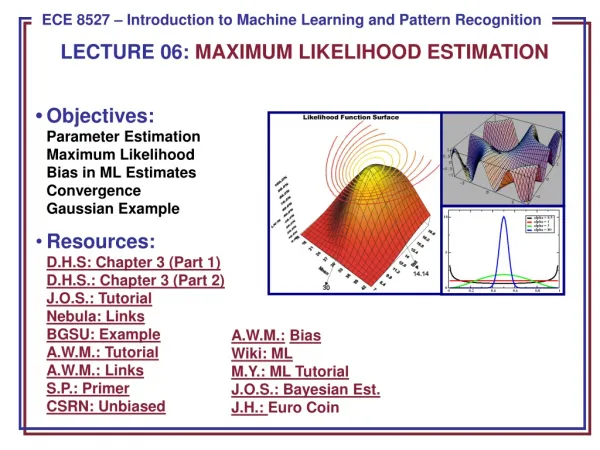
Hidden Markov Model: Extension of Markov Chains Chapter 3 (Part 3): Maximum-Likelihood and Bayesian Parameter Estimation (Section 3.10)
Hidden Markov Model (HMM) • Interaction of the visible states with the hidden states bjk= 1 for all j where bjk=P(Vk(t) | j(t)). • 3 problems are associated with this model • The evaluation problem • The decoding problem • The learning problem Pattern Classification, Chapter 3
The evaluation problem It is the probability that the model produces a sequence VT of visible states. It is: where each r indexes a particular sequence of T hidden states. Pattern Classification, Chapter 3
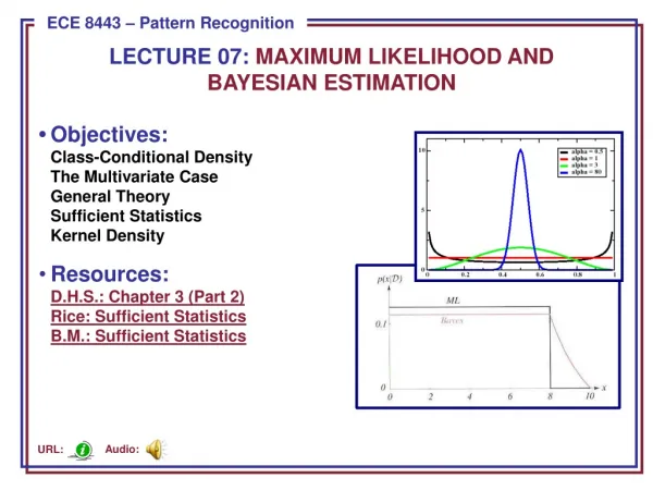
Using equations (1) and (2), we can write: Interpretation: The probability that we observe the particular sequence of T visible states VT is equal to the sum over all rmax possible sequences of hidden states of the conditional probability that the system has made a particular transition multiplied by the probability that it then emitted the visible symbol in our target sequence. Example:Let 1, 2, 3 be the hidden states; v1, v2, v3be the visible states and V3 = {v1, v2, v3} is the sequence of visible states P({v1, v2, v3}) = P(1).P(v1 | 1).P(2 | 1).P(v2 | 2).P(3 | 2).P(v3 | 3) +…+ (possible terms in the sum= all possible (33= 27) cases !) Pattern Classification, Chapter 3
v1 v2 v3 1 (t = 1) 3 (t = 3) 2 (t = 2) First possibility: Second Possibility: P({v1, v2, v3}) = P(2).P(v1 | 2).P(3 | 2).P(v2 | 3).P(1 | 3).P(v3 | 1) + …+ Therefore: v1 v2 v3 2 (t = 1) 3 (t = 2) 1 (t = 3) Pattern Classification, Chapter 3
The decoding problem (optimal state sequence) Given a sequence of visible states VT, the decoding problem is to find the most probable sequence of hidden states. This problem can be expressed mathematically as: find the single “best” state sequence (hidden states) Note that the summation disappeared, since we want to find Only one unique best case ! Pattern Classification, Chapter 3
Where: = [,A,B] = P((1) = ) (initial state probability) A = aij = P((t+1) = j | (t) = i) B = bjk = P(v(t) = k | (t) = j) In the preceding example, this computation corresponds to the selection of the best path amongst: {1(t = 1),2(t = 2),3(t = 3)}, {2(t = 1),3(t = 2),1(t = 3)} {3(t = 1),1(t = 2),2(t = 3)}, {3(t = 1),2(t = 2),1(t = 3)} {2(t = 1),1(t = 2),3(t = 3)} Pattern Classification, Chapter 3
The learning problem (parameter estimation) This third problem consists of determining a method to adjust the model parameters = [,A,B] to satisfy a certain optimization criterion. We need to find the best model Such that to maximize the probability of the observation sequence: We use an iterative procedure such as Baum-Welch or Gradient to find this local optimum Pattern Classification, Chapter 3