Download

1 / 40
400 likes | 408 Views
SPM short course – Mai 200 8 Linear Models and Contrasts. Jean-Baptiste Poline Neurospin, I2BM, CEA Saclay, France. Adjusted data. Your question: a contrast. Statistical Map Uncorrected p -values. Design matrix. images. Spatial filter. General Linear Model Linear fit

E N D
SPM short course – Mai 2008Linear Models and Contrasts Jean-Baptiste Poline Neurospin, I2BM, CEA Saclay, France
Adjusted data Your question: a contrast Statistical Map Uncorrected p-values Design matrix images Spatial filter • General Linear Model • Linear fit • statistical image realignment & coregistration Random Field Theory smoothing normalisation Anatomical Reference Corrected p-values
REPEAT: model and fitting the data with a Linear Model Plan • Make sure we understand the testing procedures : t- and F-tests • But what do we test exactly ? • Examples – almost real
One voxel = One test (t, F, ...) amplitude • General Linear Model • fitting • statistical image time Statistical image (SPM) Temporal series fMRI voxel time course
90 100 110 -10 0 10 90 100 110 -2 0 2 b2 b1 b2 = 1 b1 = 1 Fit the GLM Mean value voxel time series box-car reference function Regression example… + + =
-2 0 2 90 100 110 0 1 2 -2 0 2 b2 b1 b2 = 100 b1 = 5 Fit the GLM Mean value voxel time series Regression example… + + = box-car reference function
…revisited : matrix form b2 = b1 + + Y e = + + ´ ´ f(t) 1 b1 b2
b1 b2 Box car regression: design matrix… data vector (voxel time series) parameters error vector design matrix a = ´ + m ´ Y = X b + e
Add more reference functions ... Discrete cosine transform basis functions
…design matrix … b4 b1 b2 b3 error vector data vector + = ´ = + b Y X e
…design matrix = the betas (here : 1 to 9) parameters error vector design matrix data vector b1 a m b3 b4 b5 b6 b7 b8 b9 b2 = + ´ = + Y X b e
S = s2 the squared values of the residuals number of time points minus the number of estimated betas Fitting the model = finding some estimate of the betas raw fMRI time series adjusted for low Hz effects fitted signal Raw data fitted “high-pass filter” fitted drift residuals Noise Variance
b1 b2 b5 b6 b7 ... = + Fitting the model = finding some estimate of the betas Y = X b + e finding the betas = minimising the sum of square of the residuals ∥Y−X∥2 =Σi[ yi−Xi]2 when b are estimated: let’s call them b when e is estimated : let’s call it e estimated SD of e : let’s call it s
Take home ... • We put in our model regressors (or covariates) that represent how we think the signal is varying (of interest and of no interest alike) BUT WHICH ONE TO INCLUDE ? • Coefficients (=parameters) are estimated by minimizing the fluctuations, - variability – variance – of the noise – the residuals. • Because the parameters depend on the scaling of the regressors included in the model, one should be careful in comparing manually entered regressors
Plan • Make sure we all know about the estimation (fitting) part .... • Make sure we understand t and F tests • But what do we test exactly ? • An example – almost real
c’ = 1 0 0 0 0 0 0 0 contrast ofestimatedparameters c’b SPM{t} T = T = varianceestimate s2c’(X’X)-c T test - one dimensional contrasts - SPM{t} A contrast = a weighted sum of parameters: c´´b b1 > 0 ? Compute 1xb1+ 0xb2+ 0xb3+ 0xb4+ 0xb5+ . . . b1b2b3b4b5.... divide by estimated standard deviation of b1
Estimation [Y, X] [b, s] Y = X b + ee ~ s2 N(0,I)(Y : at one position) b = (X’X)+ X’Y (b: estimate of b) -> beta??? images e = Y - Xb(e: estimate of e) s2 = (e’e/(n - p)) (s: estimate of s, n: time points, p: parameters) -> 1 image ResMS Test [b, s2, c] [c’b, t] How is this computed ? (t-test) Var(c’b) = s2c’(X’X)+c (compute for each contrast c, proportional to s2) t = c’b / sqrt(s2c’(X’X)+c) c’b -> images spm_con??? compute the t images -> images spm_t??? under the null hypothesis H0 : t ~ Student-t( df ) df = n-p
F-test : a reduced model H0: b1 = 0 H0: True model is X0 X0 c’ = 1 0 0 0 0 0 0 0 X0 X1 F ~ (S02 - S2 ) /S2 T values become F values. F = T2 Both “activation” and “deactivations” are tested. Voxel wise p-values are halved. S02 S2 This (full) model ? Or this one?
additionalvarianceaccounted forby tested effects X0 X1 F = errorvarianceestimate F-test : a reduced model or ... Tests multiple linear hypotheses : Does X1 model anything ? H0: True (reduced) model is X0 X0 S02 S2 F ~ (S02 - S2 ) /S2 Or this one? This (full) model ?
F-test : a reduced model or ... multi-dimensional contrasts ? tests multiple linear hypotheses. Ex : does drift functions model anything? H0: True model is X0 H0: b3-9 = (0 0 0 0 ...) X0 X0 X1 0 0 1 0 0 0 0 0 0 0 0 1 0 0 0 0 0 0 0 0 1 0 0 0 0 0 0 0 0 1 0 0 0 0 0 0 0 0 1 0 0 0 0 0 0 0 0 1 c’ = This (full) model ? Or this one?
Estimation [Y, X] [b, s] Y=X b + ee ~ N(0, s2 I) Y=X0b0+ e0e0 ~ N(0, s02 I) X0 : X Reduced Test [b, s, c] [ess, F] F ~ (s0 - s) / s2 -> image spm_ess??? -> image of F : spm_F??? under the null hypothesis : F ~ F(p - p0, n-p) additionalvariance accounted forby tested effects How is this computed ? (F-test) Error varianceestimate
T and F test: take home ... • T tests are simple combinations of the betas; they are either positive or negative (b1 – b2 is different from b2 – b1) • F tests can be viewed as testing for the additional variance explained by a larger model wrt a simpler model, or • F tests the sum of the squares of one or several combinations of the betas • in testing “single contrast” with an F test, for ex. b1 – b2, the result will be the same as testing b2 – b1. It will be exactly the square of the t-test, testing for both positive and negative effects.
Plan • Make sure we all know about the estimation (fitting) part .... • Make sure we understand t and F tests • But what do we test exactly ? Correlation between regressors • An example – almost real
« Additional variance » : Again Independent contrasts
« Additional variance » : Again Testing for the green correlated regressors, for example green: subject age yellow: subject score
« Additional variance » : Again Testing for the red correlated contrasts
« Additional variance » : Again Testing for the green Entirely correlated contrasts ? Non estimable !
« Additional variance » : Again Testing for the green and yellow If significant ? Could be G or Y ! Entirely correlated contrasts ? Non estimable !
An example: real Testing for first regressor: T max = 9.8
Including the movement parameters in the model Testing for first regressor: activation is gone !
Design and contrast SPM(t) or SPM(F) Fitted and adjusted data Convolution model
Plan • Make sure we all know about the estimation (fitting) part .... • Make sure we understand t and F tests • But what do we test exactly ? Correlation between regressors • An example – almost real
C1 V A C1 C2 C3 V C2 C3 C1 C2 A C3 A real example (almost !) Experimental Design Design Matrix Factorial design with 2 factors : modality and category 2 levels for modality (eg Visual/Auditory) 3 levels for category (eg 3 categories of words)
Design Matrix not orthogonal • Many contrasts are non estimable • Interactions MxC are not modelled Asking ourselves some questions ... V A C1 C2 C3 Test C1 > C2 : c = [ 0 0 1 -1 0 0 ] Test V > A : c = [ 1 -1 0 0 0 0 ] [ 0 0 1 0 0 0 ] Test C1,C2,C3 ? (F) c = [ 0 0 0 1 0 0 ] [ 0 0 0 0 1 0 ] Test the interaction MxC ?
C1 C1 C2 C2 C3 C3 • Design Matrix orthogonal • All contrasts are estimable • Interactions MxC modelled • If no interaction ... ? Model is too “big” ! Asking ourselves some questions ... Test C1 > C2 : c = [ 1 1 -1 -1 0 0 0] V A V A V A Test V > A : c = [ 1 -1 1 -1 1 -1 0] Test the category effect : [ 1 1 -1 -1 0 0 0] c = [ 0 0 1 1 -1 -1 0] [ 1 1 0 0 -1 -1 0] Test the interaction MxC : [ 1 -1 -1 1 0 0 0] c = [ 0 0 1 -1 -1 1 0] [ 1 -1 0 0 -1 1 0]
Asking ourselves some questions ... With a more flexible model C1 C1 C2 C2 C3 C3 V A V A V A Test C1 > C2 ? Test C1 different from C2 ? from c = [ 1 1 -1 -1 0 0 0] to c = [ 1 0 1 0 -1 0 -1 0 0 0 0 0 0] [ 0 1 0 1 0 -1 0 -1 0 0 0 0 0] becomes an F test! Test V > A ? c = [ 1 0 -1 0 1 0 -1 0 1 0 -1 0 0] is possible, but is OK only if the regressors coding for the delay are all equal
Toy example: take home ... • F tests have to be used when • Testing for >0 and <0 effects • Testing for more than 2 levels in factorial designs • Conditions are modelled with more than one regressor • F tests can be viewed as testing for • the additional variance explained by a larger model wrt a simpler model, or • the sum of the squares of one or several combinations of the betas (here the F test b1 – b2 is the same as b2 – b1, but two tailed compared to a t-test).