Download
1 / 27
270 likes | 436 Views
Hyperspectral Applications Relevant to NOAA. Dr. Hsiao-hua K. Burke MIT Lincoln Laboratory GOES Users Conference 1-3 October 2002. Sponsor: NOAA NESDIS. Enhancing Operational Satellite Sensing Systems NOAA-NESDIS. Objectives (Strategic Plan 2001)

E N D
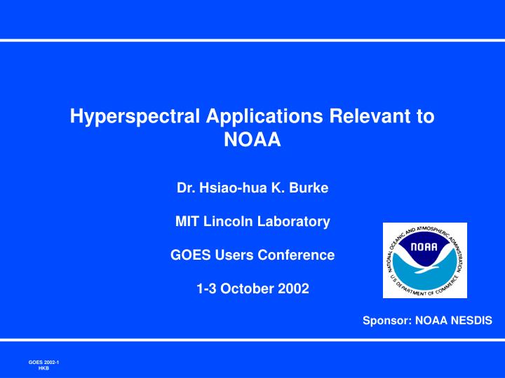
Hyperspectral Applications Relevant to NOAA Dr. Hsiao-hua K. Burke MIT Lincoln Laboratory GOES Users Conference 1-3 October 2002 Sponsor: NOAA NESDIS
Enhancing Operational Satellite Sensing SystemsNOAA-NESDIS • Objectives (Strategic Plan 2001) • “Invest in technology…. to ensure continuity improvements and new capabilities in satellite observing systems and data products” Consideration of Hyperspectral sensing as part of future NOAA observing systems
Channel Positions of Various Ocean-Color Sensors, 1978-2000* For a multi spectral sensor • Many spectral bands are identified for various applications • Selection of band location and width are also important HSI provides contiguous spectral coverage and thus comprehensive information content * IOCCG Report #1
Illustration of Enhanced Information Content from MSI to HSI Two examples shown • two similar broad bands (0.52 –0.70 and 0.52 –0.80 um) • Information contents are different • HSI allows adaptive band selection:no more competing requirements • MSI vs. HSI (EO-1 ALI and Hyperion)More feature information availabledespite lower SNR of Hyperion 0.52-0.70 mm 0.52-0.80 mm ALI Hyperion
Principal Components Analysis (PCA)- Reduction of HSI Dimensionality - Principal Components Transform • A linear transform that projects data onto an orthogonal set of basis functions that are eigenvectors of the spectral covariance matrix: Covariance Matrix: S= E{(X - M)(X - M)T} Eigenvectors and Eigenvalues: Se= L e Apply to Image Cube: PC(x,y)= eT X(x,y) • Standard multivariate analysis technique • Dimensionality reduction • Contrast enhancement • Anomaly detection • Separates significant scene information from noise dominated components • large eigenvalues ->components that greatly contribute to overall variance • small eigenvalues -> noise dominated components
Principal Components Analysis (PCA)- Reduction of HSI Dimensionality - Cont. Eigenvalues • Indicative of the amount of spectral variability represented by corresponding eigenvector large values àscene components that greatly contribute to overall variance small values ànoise dominated components intermediate valuesß? anomalous features Eigenstructure Computed from example imagery Eigenvectors PC: 12345 • “Groups” spectral channels that have similar contributions to overall spectral variability • Ordered by decreasing eigenvalue • Can help to identify important spectral regions Full spectral information can be recovered
An Illustration:Similar Bands, Different Information Content Broad Images 0.52-0.70 mm 0.52-0.80 mm Images simulated by integrating (18 & 28) AVIRIS HSI bands Animation to follow
Broad Images PC 1 PC 2 PC 3 PC 4 PC 5 PC 6 PC 7 PC 8 PC 9 PC 10 An Illustration:Similar Bands, Different Information Content 0.52-0.70 mm 0.52-0.80 mm
Cascaded Principal Component AnalysisMinimum Noise Fraction (MNF) Transform • Principal Components Transformation (PCT) • Covariance Matrix: S = E {(C - Cm)(C - Cm)T} • Eigenvectors and Eigenvalues: S = F L FT • MNF: Two cascaded PCTs • The first based on estimated noise covariance • Band-to-band de-correlated noise in transformed data • The second PCT on noise-whitened data • Unit noise variance • Result: • Image information aggregated in leading components • Noise segregated in trailing components • Inherent dimensionality of HSI data determined
EO-1 Data from Chesapeake Bay Selected area (~6 x 15 km2), 0.43 to 0.93 mm only • ALI • 200 samples/line • 512 lines • 6 bands • (MS-1’,1,2,3,4,4’) • Hyperion • 194 samples/line • 496 lines • 50 bands • (0.43-0.93 mm)
MNF Bands 1 & 2 ALI MNF Band 1 Hyperion MNF Band 1 ALI MNF Band 2 Hyperion MNF Band 2 Animation to follow
MNF Components for ALI and Hyperion ALI MNF 5 ALI MNF 4 ALI MNF 2 ALI MNF 6 Hyperion MNF 1 Hyperion MNF 3 Hyperion MNF 13 Hyperion MNF 12 Hyperion MNF 11 Hyperion MNF 9 Hyperion MNF 8 Hyperion MNF 14 Hyperion MNF 5 Hyperion MNF 10 Hyperion MNF 7 ALI MNF 3 ALI MNF 1 Hyperion MNF 2 Hyperion MNF 4 Hyperion MNF 6
Example Spectral Products 4 – 8m Temperature profile Water vapor profile Water vapor winds at altitudes Surface characteristics Climate monitoring 8-15 m Temperature profile Cloud properties Cloud winds Storms Trace gases (Volcanic SO2, O3) Surface temperature Radiation Climate monitoring .4 – 2.5m Ocean color/ bathymetry Integrated water vapor Cloud top estimate Aerosol optical depth, type & dynamics Volcanic SO2 monitoring Climate monitoring • Overall HSI Benefits • Provide data as a dynamic spectral shell • Match the spectral domain – hyperspectral • Satellite-to-satellite calibrationChannel selectivityNoise reductionStable climate recordAlgorithm transferability and growthSystem backup
“Own the Spectrum” • Hyperspectral technology demonstrated on A/C and space • Enabled by large focal plane technology, processing capability • 0.4-2.5 mm (210 bands): AVIRIS, Hyperion • 2- 6 mm (75 bands) ARES, 3-5 mm (128 bands) SEBASS • 8-14 mm (128 bands) SHARP • NAST-I, AIRS • However, in addition to “spectral”, there are also requirements for • Spatial (resolution, coverage) • Temporal (revisit, rapid scan) • Radiometric (SNR) not to mention • Data volume, comm, processing constraints Explore system approach to optimize new technology and maximize weather, climate, ocean and environmental utility for future NOAA sensor systems
Examples of HSI Applications • Coastal Characterization • Chlorophyll content • Atmospheric characterization • Integrated water vapor • Cloud/plume surface depiction • Cloud top altitude determination
Why HSI for Coastal Characterization? • Most ocean feature algorithms are semi-empirical retrievals, HSI has all bands to: • Provide legacy with previous sensors • Explore new information • Coastal features are more complex than those of deep (open) ocean • Coupled effects best resolved with HSI • With contiguous spectral coverage, atmospheric compensation can be done with more accuracy and confidence • Most ocean characterization algorithms utilize water-leaving radiance • Aerosol effect most pronounced in shortwave visible where ocean color measurements are made
Chlorophyll-a Calculations (HYPERION) 478nm 600nm 447nm 478nm 488nm 600nm 529nm 763nm 550nm Line 64 Line 64 Line 225 Line 64 Line 225 -64 531nm763nm .04 -225 Line 400 Line 475 Line 400 Line 475 .02 -400 Range: 2.1 to 3.6 mg/m3 Calculated using SeaWIFS OC4 -475
Supporting Data Chesapeake Bay Remote Sensing Program CBRSP 2/19/02 SeaWIFS Data averaged for the week 2/18/02-2/25/02 Chlorophyll-a immediately inside the Bay is between 2 to 4 mg/m3. EO-1 data area is shown in red box 2.0 to 4.0 mg/m3(Level 3 calculations use OC4 algorithm) • Initial chlorophyll retrieval from Hyperion data demonstrated: • good agreement with published data
HSI Water Vapor Retrieval Using NIR Water Vapor Transmission NIR Water Vapor Band Ratios For a given narrow absorption band, ratioing between band center and wings provides an estimate of the total integrated water vapor value
Example of Water Vapor Retrieval- AVIRIS Moffett Field Scene - E. San Francisco BayRGB Image Retrieved Water Vapor Map 1.2 1.0 0.8 0.6 0.5-0.7 cm Column Water Vapor (cm) 1.0-1.2 cm 1.0-1.2 cm 0.5-0.7 cm Top Bottom 10 km AVIRIS scene collected near Milpitas CA with the San Francisco Bay off to the left side. Bright color indicates higher concentrations. Orographic effects on the distribution of water vapor are clearly visible.
Cloud/Plume/Fire Scene Characterization AVIRIS Image Cube • Smoke • Dense plume • Thin plume • Surface features observed • Active fire • Burning zones and hot spots • Cloud • Discriminate from smoke • Burn assessment • Extent of burnt vegetation • Modify operational approach to work better in haze environment l : 400 – 2500 nm
AVIRIS Image - Linden CA 20-Aug-1992 224 Spectral Bands: 0.4 - 2.5 mm Pixel: 20mx 20mScene: 10km x 10km Spectral Signatures Feature Spectral Information
Exploitation of Spectral InformationID and Assessment of Cloud/Plume/Burn Damage Burn Index Cloud Cloud and Thick Smoke Mask Smoke large part. Smoke - small part. Ref (1100) - Ref (2200) Ref (1100) + Ref (2200) B.I. = Hot Area Potential of HSI application to environment characterizationis demonstrated Use spectral channel combinations to depict cloud/plume domains
SCAR-B Cloud Scene A Cloud spectra are fairly uniform throughout the scene Clouds As Shadow B Bs AVIRIS SCAR-B, 20 August 1995
Cloud Top Height Retrieved Using Depth of Water Vapor Absorption Bands 0.94 mm channel 1.14 mm channel 1.4 mm channel 1.9 mm channel • 0.94 and 1.14 mm regions are useful for low and middle level clouds • 1.4 and 1.9 mm regions are opaque near surface and useful for high level clouds ChannelApparent ReflectanceHeight 0.94 mm 0.54 3.9 km 1.14 mm 0.42 3.9 km Water Vapor Method Cloud Top Height ~ 3.9 km
Conclusion The promise of Hyperspectral sensing for NOAA • Provide data as a dynamic spectral shell • Match the spectral domain – hyperspectral Satellite-to-satellite calibration Channel selectivity Noise reduction Stable climate record Algorithm transferability and growth System backup The challenge: Explore system approach to optimize new technology and maximize weather, climate, ocean and environmental utility for future NOAA sensor systems