Mathematical Morphology
Mathematical Morphology. Mathematical morphology (matematická morfologie) A special image analysis discipline based on morphological transformations of the image (usually a binary image). Developed: In early 1980’s by the group of Jean Serra Centre de Morphologie Mathématique (CMM)


Mathematical Morphology
E N D
Presentation Transcript
Mathematical Morphology • Mathematical morphology (matematická morfologie) • A special image analysis discipline based on morphological transformations of the image (usually a binary image). • Developed: In early 1980’s by the group of Jean Serra Centre de Morphologie Mathématique (CMM) Fontainebleau, France http://www.ensmp.fr/Eng/Research/Domain/MathInfoAuto/CMM/CMM.html http://cmm.ensmp.fr/Recherche/recherche_eng.htm • Motivation: Binary image (obtained e.g. using thresholding or edge detection followed by edge linking and object filling) often needs further processing such as overlapping object separation, filling of holes, removal of narrow protrusions and other morphological (i.e. shape) changes.
Mathematical Morphology • Principles: • Such further processing is performed using one or a combination of several morphological transformations. • The transformations work in a certain local neighborhood of each pixel (similarly to convolution) defined by so called structuring element (strukturní element). The structuring element can be square, cross-like or any other shape. • There are two types of morphological transformations: binary and grey-scale. Binary transformations transform binary images into binary images. Grey-scale transformations transform grey-scale images into grey-scale images.
Mathematical Morphology: Binary Images • Dilation (dilatace) • Dilation replaces zeros neighboring to ones by ones. • Erosion (eroze) • Erosion replaces ones neighboring to zeros by zeros. • Closing (uzavření) • Closing is dilation followed by erosion. • Closing merges dense agglomerations of ones together, fills small holes and smoothes boundaries. • Opening (otevření) • Opening is erosion followed by dilation. • Opening removes single ones, thin lines and divides objects connected with a narrow path (neck).
Mathematical Morphology: Binary Images Original Erosion with a 3x3 mask Opening with a 3x3 mask Opening with a 5x5 mask
Mathematical Morphology: Binary Images Original Dilation with a 3x3 mask Closing with a 3x3 mask Closing with a 5x5 mask
Mathematical Morphology: Binary Images Opening + Closing (3x3 mask) Opening + Closing (5x5 mask) Closing + Opening (3x3 mask) Closing + Opening (5x5 mask)
Mathematical Morphology: Binary Images • Shrinking (”zcvrkávání”) • Shrinking is a modification of erosion: object without holes erodes to a single pixel at or near its center of mass, object with holes erodes to a connected ring lying midway between each hole and its nearest outer boundary. • Thinning (ztenčování) • Thinning is a modification of erosion: object without holes erodes to a minimally connected stroke located equidistant from its nearest outer boundaries, object with holes erodes to a minimally connected ring lying midway between each hole and its nearest outer boundary. • Skeletonizing (vytváření skeletu neboli kostry) • Skeletonizing is a modification of erosion: object erodes to a set of points that are equally distant from two closest points of an object boundary (this set of points is also called medial axis skeleton). Skeleton uniquely describes the structure of the object.
Mathematical Morphology: Grey-scale Images • Dilation (dilatace) • Dilation replaces the central pixel with the maximum of its neighbors. • Erosion (eroze) • Erosion replaces the central pixel with the minimum of its neighbors. • Closing (uzavření) • Closing is dilation followed by erosion. • Closing merges dense agglomerations of local maxima together, fills small holes and smoothes boundaries. • Opening (otevření) • Opening is erosion followed by dilation. • Opening removes single local maxima, thin lines and divides objects connected with a narrow path (neck).
Watershed Algorithm • Developed: 1978 by Ch. Lantuéjoul (CMM, Fontainebleau, France) 1979 by S. Beucher (CMM, Fontainebleau, France) Ch. Lantuéjoul, PhD thesis, CMM, 1978 http://cmm.ensmp.fr/~beucher/wtshed.html • Idea: Flood simulation by increasing the water level step by step.The grey-scale image is considered as a topographic surface.Creation of catchment basins and watershed lines.
Watershed Algorithm • Method: • Image smoothing (usually Gaussian filter),the kernel size depends on object size and also on noise. • Determination of maximum intensity (MaxI) andminimum intensity (MinI) of the whole image. • Determination of so-called markers, i.e. seeds of future objects. Can be performed e.g. using a minimum filter. • Binary image (BinImg) = empty image (zeros) • For CurI = MinI to MaxI doPerform region growing from markers (or already existing regions of BinImg) so that all pixels with intensities lower or equal to CurI are included. Do not let the regions merge! • BinImg now defines object territories. The number of objects is equal to the number of markers.
Watershed Algorithm • Notes: • The algorithm can work without markers, in this case markers are all local minima in the image (in 3x3 neighborhood). • Markers can be determined manually or automatically using better approaches than minimum filter, e.g. using distance transform – the image is thresholded (bilevel thresholding), boundaries are determined and the shortest distance of each pixel to the closest boundary point is determined. Those pixels which have large distance to the boundary (larger than a pre-defined threshold) are taken as markers. • The loop can be performed also from MaxI down to MinI for inverted images (bright objects and dark background). This approach is called anti-watershed. • The algorithm is usually applied to gradient image (Sobel image) in order to detect object boundaries.
Watershed Algorithm Example of the determination of markers and watershed Original grey-scale Thresholding (green) Watershed result Distance transform Segmentation (red) Markers (red) Markers (black)
Largest Contour Segmentation (LCS) • Developed: 1996 by E.M.M.Manders (Delft, The Netherlands) Cytometry 23: 15-21 (1996) • Idea: Iterative region growing around each local intensity maximum.Works on 2D as well as 3D images.
Largest Contour Segmentation (LCS) The Method 1) Noise filtering (average or median),the kernel size depends on noise type and magnitude. 2) Determination of local maxima and minimal intensity in the image (GlobalMinI) 3) Calculation of centers of local maxima, i.e. reduction of local maxima to 1 pixel. 4) For each local maximum do 4.1) Current threshold (CurT) = (Max intensity (LocalMaxI) + GlobalMinI) / 2 4.2) Number of iterations (I) = 0 4.3) Perform region growing from the center of the local maximum so that all neighboring pixels are included whose intensity values CurT. 4.4) N = the number of centers inside this region. 4.5) I = I + 1 4.6) If I = BitDepth, finish iteration for the given center and go to step 5. 4.4) If N>1, CurT = (CurT + previous higher threshold) / 2 4.5) If N=1, CurT = (CurT + previous lower threshold) / 2 4.6) Go to step 4.3. 5) If N>1, Final threshold (FinT) = CurT+1If N=1, Final threshold (FinT) = CurT
Largest Contour Segmentation (LCS) Example Original grey-scale Gaussian filter 7x7 Centers of local maxima GlobalMinI=27 LocalMaxI=207 (left top) LocalMaxI=183 (bot. right)
Largest Contour Segmentation (LCS) Example (continued for the bottom right cell) Input CurT=105 CurT=144 CurT=163 CurT=153 CurT=158 CurT=160 CurT=161 CurT=162 FinT=162