Download
1 / 38
430 likes | 678 Views
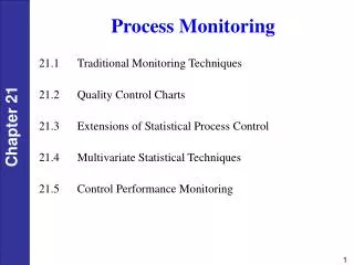
Model Based Process Monitoring Methods. Model-Based. Residual based observers Parity-space based Causal models Signed digraphs. Statistical. PCA PLS. Process monitoring methods. Process monitoring. + Includes process knowledge − Needs process models. + Easier to implement

E N D
Model-Based Residual based observers Parity-space based Causal models Signed digraphs Statistical PCA PLS Process monitoring methods Process monitoring + Includes process knowledge − Needs process models + Easier to implement − Don’t include process knowledge Data-Based Quantitative Qualitative Rule-based (Fuzzy) Neural Networks introductory Scope of the course PCA PLS + GA and some Control
Topics • 1. Causal model (Qualitative model) based method • 2. Noise residual detection method • 3.Analytical FDI methods (Quantitative mathematic model) • Observer based method • Parameter estimation method
The causal digraph model (CDG) • The causal digraph is defines as: CDG=(nodes, arcs, values of nodes, model of arcs) • Causal Digraph knowledge representation • Nodes interesting variables • Arc cause – effect relations (e.g. state space model) • Direction The direction of causality (from input variable to output variable) • The model can be obtained both from history data or a mathematical model Cause-effect model Process variables Cause-effect model Pipe fluid model Pump rotation Tank material balance model Tank level Mass flow rate Valve opening
1 3 6 4 2 5 The Causal directed graph with state space model What would be the structure of a state space model between node 3 and it’s input nodes if we assume that node 3 has 2 states (but one output)?
The Causal directed graph with state space model • General fault detection and isolation procedure with causal digraph model • Residual generation: generate a signal which is only sensitive to the fault • Residual evaluation : detect changes in the residual signal and fire the alarm • Decision making : analyze the alarm pattern to locate the fault origin
Fault detection and isolation • Causal Digraph residual generation • Global residual • Local residuals • Individual local residuals • Multiple local residuals • Total local residuals
10 7.4 1223 98 Process variables 1.23 Measurements for control 66 Fault detection and isolation • Causal digraph residual generation • Global residual generation No measurements are used except for the boundary signals Actuator signals
Fault detection and isolation • Causal Digraph residual generation • Local residuals • Individual local residuals Global propagation value one measurement is used Measured value Global propagation value
Fault detection and isolation • Causal Digraph residual generation • Local residuals • Individual local residuals • Multiple local residuals Global propagation value Measured values some measurements are used Global propagation value
Fault detection and isolation • Causal Digraph residual generation • Local residuals • Individual local residuals • Multiple local residuals • Total local residuals Measured value Only measured values are used
Fault detection and isolation • The reason for calculating residuals with several measured variables is that it makes the detection of fault propagation via multiple paths possible. If we are using only individual local residuals some faults cannot be isolated. • How many residuals have to calculated if a node has 3 input?
Fault detection and isolation • The number of residuals for n inputs can be calculated generally as • This is one drawback of this method. Computationally demanding to calculate so many residuals
Fault detection and isolation • Causal Digraph residual evaluation • The generated residual signals needs to be mapped to the set {0,1} • For instance the CUSUM method can be used for this task (to be presented later)
Fault detection and isolation • Simple illustration (f=model) Inference rules • GR = y2mes− f(θ, u1glob) • LR = y2mes − f(θ, u1mes) 2 1 3 Assumption: no simultaneous faults! Residuals for node 2 GR2 LR2 Residuals for node 3 GR3 LR3 y2,globθ3 y3,mes y2,mes y1,globθ2 y2,mes y1,mes If residuals 1 1 fault in y2,mes or θ2 if residuals 1 0 fault y1,globif residuals 0 1 fault y1,mes
GR GR 1 1 LR(1,2) LR 0 0 3 GR 1 2 LR(1) 1 LR(2) 0 Example 1Process variable fault 1 3 4 2
1 1 1 3 3 3 4 4 2 2 2 2 Example 2 Process fault Manipulated Variable Process Varaible1 Process Varaible2 Controlled Variable Process 2 4 4 3 3 4 1 0.5 12 16 Static model Static model GlobalModel Static model 3 2 4 3 4 3 12 1 0.5 Static model Predicted value LocalModels Legend 2 0.5 1 Measurement 3 Fault Origin 3 1 4 Propagated fault 12 16 3 4
GR 0 LR GR 0 0 3 GR 1 2 LR(2) 1 LR(1,2) LR(1) 1 0 GR 0 Example 3Measurement fault 1 4 3 2
1 1 1 3 3 3 4 2 2 2 2 Example 4Measurement fault Manipulated Variable Process Varaible1 Process Varaible2 Controlled Variable Process 2 4 3 3 4 1 0.5 12 Static model Static model GlobalModel Static model 3 2 4 3 4 3 12 1 0.5 Static model Predicted value LocalModels Legend 2 0.5 1 Measurement 3 Fault Origin 3 1 4 Propagated fault 4 12 16 3 4
Fault detection and isolation • General rules • Fault location rules • Fault nature rules
Fault detection and isolation General rules • Fault locationrules • Fault nature rules
CDG - Case study • Description of short circulation process in a paper machine
CDG - Case study • Importance of the short circulation process: • The dilution of the fibre-suspension entering the process to a suitable consistency for the headbox (mixing process of low-consistency water from the wire-pit is mixed with high-consistency stock) • The removal of impurities and air. This task is performed in the hydro-cyclones, machine screens and the so-called deculator. • The short circulation also improves the economy of the process because the valuable fibres and filler materials that pass through the wire are recycled. • As the intermediate process between stock preparation and former, the short circulation process is very important for paper quality control, since the basic weight, ash and jet ratio control are performed in the short circulation part.
CDG - Case study • Flow sheet of the process
CDG - Case study • Faulty case • The grade of paper machine • Basic weigh: 50g/m2 • Ash rate: 18% • Moisture: 7% • The operation point • Basic valve opening: 0.25 • Filler valve opening: 0.5 • Head box stock feed pump: 75.2% • Head box slice opening: 10mm • The artificial faults • Consistency sensor fault: a 3.5e−6%/s drift is added to the measurement (1800−7800 s ) • Process fault: The retention of filler on wire drops from 50% to 45% (8800−17800 s)
Case study - Causal Model Construction • Select variables and construct the graph structure
Case study - Causal Model Construction • Identify the cause-effect relations between variables • Training and validation data were collected from the APROS (VTT) paper making simulator under the fault free state • NNDT (Neural Network development Tool) was used to identify the state space models
Case study - The result of test • Global residuals
Case study - The result of test • Result for the consistency sensor fault
Case study - The result of test • Result for the retention drop process fault
Case study - Conclusion • Conclusion • The method was able to locate the fault using the general inference rules • The method was able to tell the nature of the fault • The method was difficult to implement while it provides quite rich information to the operator
Page Hinkley CUSUM test • Earlier in the course we have introduced several methods that will generate a residual as a monitoring result. • In practical applications this signal can be very noisy and the use of a simple threshold to detect changes in the residual might not give satisfactory results • The CUSUM method by Page-Hinkley offers a solution to this problem
Page Hinkley CUSUM test • The method is based on the calculation of a cumulative sum • Algorithm: • detection when: μ0: signal mean ν: minimum detectable jump λ: detection threshold
Code my0 = 0; lamda = 1; minfault = 0.4; m_n = 1E6; summ = 0; for i = 1 : length(y), summ = summ + (y(i)-my0-minfault/2); sumsave(i) = summ; if sumsave(i) < m_n m_n = sumsave(i); end g = summ-m_n; if g >= lamda alarm(i) = 1; else alarm(i) = 0; end end
CUSUM example Let’s study the following signal! It’s difficult to say much about this residual just by looking
CUSUM example • If we use a simple threshold (0.45) we get the following alarm sequence Alarm = 1 if y > 0.45 Else Alarm = 0
CUSUM example • If we use the CUSUM method we get the following results. A continuous alarm signal without much delay (the fault actually happened at t = 50). The lower figure illustrates the cumulative sum