Download
1 / 30
300 likes | 443 Views
Multiple View Geometry. Marc Pollefeys University of North Carolina at Chapel Hill. Modified by Philippos Mordohai. Tutorial outline. Introduction Visual 3D modeling Acquisition of camera motion Acquisition of scene structure Constructing visual models Examples and applications .

E N D
Multiple View Geometry Marc Pollefeys University of North Carolina at Chapel Hill Modified by Philippos Mordohai
Tutorial outline • Introduction • Visual 3D modeling • Acquisition of camera motion • Acquisition of scene structure • Constructing visual models • Examples and applications
Visual 3D models from images “Sampling” the real world • Visualization • Virtual/augmented/mixed reality, tele-presence, medicine, simulation, e-commerce, etc. • Metrology • Cultural heritage and archaeology, geology, forensics, robot navigation, etc. Convergence of computer vision, graphics and photogrammetry
Visual 3D models from video What can be achieved? unknown scene unknown camera Scene (static) camera unknown motion automatic modelling Visual model
Example: DV video 3D model accuracy ~1/500 from DV video (i.e. 140kb jpegs 576x720)
(Pollefeys et al. ICCV’98; … Pollefeys et al.’IJCV04)
Outline • Introduction • Image formation • Relating multiple views
Perspective projection Perspective projection Linear equations (in homogeneous coordinates)
m M1 C M2 Homogeneous coordinates • 2-D points represented as 3-D vectors (x y 1)T • 3-D points represented as 4-D vectors (X Y Z 1)T • Equality defined up to scale • (X Y Z 1)T ~ (WX WY WZ W)T • Useful for perspective projection makes equations linear
Effects of perspective projection • Colinearity is invariant • Parallelism is not preserved
Intrinsic parameters • Camera deviates from pinhole s: skew fx ≠ fy: different magnification in x and y (cx cy): optical axis does not pierce image plane exactly at the center • Usually: rectangular pixels: square pixels: principal point known: or
Extrinsic parameters Scene motion Camera motion
Projection matrix • Includes coordinate transformation and camera intrinsic parameters
Projection matrix • Mapping from 2-D to 3-D is a function of internal and external parameters
Radial distortion • In reality, straight lines are not preserved due to lens distortion • Estimate polynomial model to correct it
Outline • Introduction • Image formation • Relating multiple views
L2 M? M Triangulation m2 l2 C2 3D from images m1 C1 L1 • calibration • correspondences
Comparing image regions Compare intensities pixel-by-pixel I(x,y) I´(x,y) (Dis)similarity measures Normalized Cross Correlation • Sum of Square Differences
Feature matching Multi-view relation Structure and motion recovery Self-calibration Structure and motion recovery Feature extraction
Other cues for depth and geometry Shading Shadows, symmetry, silhouette Texture Focus
P P L2 L2 m1 m1 m1 C1 C1 C1 M M L1 L1 l1 l1 e1 e1 lT1 l2 e2 e2 l2 m2 m2 m2 l2 l2 Fundamental matrix (3x3 rank 2 matrix) C2 C2 C2 Epipolar geometry Underlying structure in set of matches for rigid scenes • Computable from corresponding points • Simplifies matching • Allows to detect wrong matches • Related to calibration
The epipoles The epipole is the projection of the focal point of one camerain another image. e21 e12 C2 C1 Image 2 Image 1
Two view geometry computation:linear algorithm • For every match (m,m´):
Benefits from having F • Given a pixel in one image, the corresponding pixel has to lie on epipolar line • Search space reduced from 2-D to 1-D
Matching difficulties • Occlusion • Absence of sufficient features (no texture) • Smoothness vs. sensitivity • Double nail illusion
Two view geometry computation:more problems • Repeated structure ambiguity • Robust matcher also finds • support for wrong hypothesis • solution: detect repetition