Download

1 / 74
2.23k likes | 4.57k Views
PTT 204/3 APPLIED FLUID MECHANICS SEM 2 (2012/2013). Chapter 8 : Flow in Pipes (Internal Flow). Objectives. Have a deeper understanding of laminar and turbulent flow in pipes and the analysis of fully developed flow

E N D
PTT 204/3APPLIED FLUID MECHANICSSEM 2 (2012/2013) Chapter 8: Flow in Pipes (Internal Flow)
Objectives • Have a deeper understanding of laminar and turbulent flowin pipes and the analysis of fully developed flow • Calculate the major and minor losses associated with pipeflow in piping networks and determine the pumping powerrequirements • Understand various velocityand flow rate measurementtechniques and learn theiradvantages and disadvantages
8–1 ■INTRODUCTION • Liquid or gas flow through pipesor ductsis commonly used in heating andcooling applications and fluid distribution networks. • The fluid in such applicationsis usually forced to flow by a fan or pumpthrough a flow section. • We pay particular attention to friction, which is directly related to the pressuredropand head lossduring flow through pipes and ducts. • The pressuredrop is then used to determine the pumping power requirement. Circular pipes can withstand largepressure differences between theinside and the outside withoutundergoing any significant distortion,but noncircular pipes cannot.
Internal flows through pipes, elbows, tees,valves, etc., as in this oil refinery, are foundin nearly every industry.
8–2■LAMINAR AND TURBULENT FLOWS Laminar flow is encounteredwhen highly viscous fluids such as oils flow in small pipes or narrowpassages. Laminar:Smooth streamlines and highly ordered motion. Turbulent:Velocity fluctuations and highly disorderedmotion. Transition:The flow fluctuatesbetween laminar and turbulent flows. Mostflows encountered in practice are turbulent. The behavior of colored fluid injectedinto the flow in laminar and turbulentflows in a pipe. Laminar and turbulent flow regimesof candle smoke plume.
Reynolds Number At large Reynolds numbers, the inertial forces, which are proportional to the fluid density and the square of the fluid velocity, are large relative to the viscous forces, and thus the viscous forces cannot prevent the random and rapid fluctuations of the fluid (turbulent). At small or moderate Reynolds numbers, the viscous forces are large enough to suppress these fluctuations and to keep the fluid “in line” (laminar). The transition from laminar to turbulent flow depends on the geometry,surfaceroughness, flow velocity, surface temperature, and type of fluid. The flow regime depends mainly on the ratio of inertialforcesto viscous forces(Reynolds number). Critical Reynolds number, Recr:The Reynolds number at which the flow becomes turbulent. The value of the critical Reynolds number is different for different geometries and flow conditions. The Reynolds number can be viewedas the ratio of inertial forces to viscousforces acting on a fluid element.
For flow through noncircular pipes, the Reynolds number is based on the hydraulic diameter For flowin a circular pipe: The hydraulic diameter Dh = 4Ac/p isdefined such that it reduces to ordinarydiameter for circular tubes. In the transitional flow regionof 2300 Re4000, the flowswitches between laminar andturbulent seemingly randomly.
8–3■THE ENTRANCE REGION Velocity boundary layer:The region of the flow in which the effects of the viscous shearing forces caused by fluid viscosity are felt. Boundary layer region:The viscous effects and the velocity changes are significant. Irrotational (core) flow region:The frictional effects are negligible and the velocity remains essentially constant in the radial direction. The development of the velocityboundary layer in a pipe. Thedeveloped average velocity profile isparabolic in laminar flow,but somewhat flatter or fuller inturbulent flow.
Hydrodynamic entrance region:The region from the pipe inlet to the point at which the boundary layer merges at the centerline. Hydrodynamic entry length Lh:The length of this region. Hydrodynamically developing flow:Flow in the entrance region. This is the region where the velocity profile develops. Hydrodynamically fully developed region:The region beyond the entrance region in which the velocity profile is fully developed and remains unchanged. Fully developed:When both the velocity profile and the normalized temperature profile remain unchanged. Hydrodynamically fully developed In the fully developed flow region ofa pipe, the velocity profile does notchange downstream, and thus the wallshear stress remains constant as well.
The pressure drop is higher in theentrance regions of a pipe, and the effect of theentrance region is always toincrease the averagefriction factor for the entire pipe. The variation of wall shear stress inthe flow direction for flow in a pipe from the entrance region into the fullydeveloped region.
Average velocity Vavg is defined as theaverage speed through a cross section.For fully developed laminar pipe flow,Vavg is half of the maximum velocity.
Entry Lengths The hydrodynamic entry length is usually taken to be the distance from thepipe entrance to where the wall shear stress (and thus the friction factor)reaches within about 2 percent of the fully developed value. hydrodynamic entry length for laminar flow hydrodynamic entry length for turbulent flow hydrodynamic entry length for turbulent flow, an approximation
8–4■LAMINAR FLOW IN PIPES We consider steady, laminar, incompressible flow of a fluid with constantproperties in the fully developed region of a straight circular pipe. In fully developed laminar flow, each fluid particle moves at a constant axialvelocity along a streamline and the velocity profile u(r) remains unchanged inthe flowdirection. There is no motion in the radial direction, and thus thevelocitycomponent in the direction normal to the pipe axis is everywhere zero.There is no acceleration since the flow is steady and fully developed. Free-body diagram of a ring-shapeddifferential fluid element of radius r,thickness dr, and length dx orientedcoaxially with a horizontal pipe infully developed laminar flow.
Boundary conditions Average velocity Velocity profile Maximum velocity at centerline Free-body diagram of a fluid diskelement of radius R and length dx infully developed laminar flow in ahorizontal pipe.
Pressure Drop A quantity of interest in the analysis of pipe flow is the pressure drop ∆P since it is directly related to the power requirements of the fan or pump to maintain flow. A pressure drop due to viscouseffects represents an irreversible pressure loss, and it is called pressure lossPL. Pressure loss for all types offully developed internal flows (laminar/ turbulent flows, circular/ non-circular pipes, smooth/ rough surfaces, and horizontal or inclined pipes) Darcy friction factor Dynamic pressure Circular pipe, laminar In laminar flow, the friction factor is a function ofthe Reynolds number only and is independent of the roughness of the pipesurface.
Head Loss and Pumping Power The head lossrepresents the additional height that the fluid needs to beraised by a pump in order to overcome the frictional losses in the pipe. Head loss (laminar/turbulent flows, circular/non-circular pipes) The relation for pressure loss (andhead loss) is one of the most generalrelations in fluid mechanics, and it isvalid for laminar or turbulent flows,circular or noncircular pipes, andpipes with smooth or roughsurfaces. The required pumping power to overcome the pressure loss.
Laminar Flow (Horizontal pipe) Poiseuille’s law For aspecified flow rate, the pressure drop and thus the required pumping poweris proportional to the length of the pipe and the viscosity of the fluid, but it isinversely proportional to the fourth power of the diameterof thepipe.
The pressure dropP equals the pressure loss PLin the case of a horizontalpipe, but this is not the case for inclined pipes or pipes with variablecross-sectional area. This can be demonstrated by writing the energy equationfor steady, incompressible one-dimensional flow in terms of heads as
Effect of Gravity on Velocity and Flow Rate inLaminar Flow Laminar Flow (Inclined pipe) Free-body diagram of a ring-shapeddifferential fluid element of radius r,thickness dr, and length dx orientedcoaxially with an inclined pipe in fullydeveloped laminar flow.
Laminar Flow in Noncircular Pipes The friction factor f relations are given in Table 8–1 for fully developed laminar flow in pipes of various cross sections. The Reynolds number for flow in these pipes is based on the hydraulic diameter Dh = 4Ac/p, where Acis the cross-sectional area of the pipe and p is its wetted perimeter
8–5 ■TURBULENT FLOW IN PIPES Most flows encountered in engineering practice are turbulent, and thus it isimportant to understand how turbulence affects wall shear stress. Turbulent flow is characterized bydisorderly and rapid fluctuations ofswirling regions of fluid, called eddies, throughout the flow. These fluctuationsprovide an additional mechanism for momentum and energy transfer. In turbulent flow, the swirling eddiestransport mass, momentum,and energy to other regions of flow much more rapidlythan molecular diffusion,greatly enhancing mass, momentum, and heat transfer. As a result,turbulent flow is associated with much higher values of friction, heat transfer,and mass transfer coefficients The intense mixing in turbulent flowbrings fluid particles at differentmomentums into close contact andthus enhances momentum transfer.
The laminar component:accounts for the friction between layers in the flow direction The turbulent component:accounts for the friction between the fluctuating fluid particles and the fluid body (related to the fluctuation components of velocity). Fluctuations of the velocity component u with time at a specified location in turbulent flow. The velocity profile and the variation of shear stress with radial distance for turbulent flow in a pipe.
Turbulent Velocity Profile Thevery thin layer next to the wall where viscous effects are dominant is theviscous(orlaminaror linearor wall) sublayer. The velocity profile in thislayer is very nearly linear, and the flow is streamlined. Next to the viscoussublayer is the buffer layer, in which turbulent effects arebecoming significant,but the flow is still dominated by viscous effects. Above the bufferlayer is the overlap(or transition) layer, also called the inertial sublayer,in which the turbulent effects are much more significant, but still not dominant. Above that is the outer(or turbulent) layerin the remaining part ofthe flow in which turbulent effects dominate over molecular diffusion (viscous)effects. The velocity profile in fully developedpipe flow is parabolic in laminar flow,but much fuller in turbulent flow.
The Moody Chartand theColebrook Equation Colebrook equation (for smooth and rough pipes) The friction factor in fully developed turbulent pipe flow depends on theReynolds number and the relative roughness /D. Explicit Haaland equation The friction factor is minimum fora smooth pipe and increases withroughness.
Observations from the Moody chart • For laminar flow, the friction factor decreases with increasing Reynolds number, and it is independent of surface roughness. • The friction factor is a minimum for a smooth pipe and increases with roughness. The Colebrook equation in this case ( = 0) reduces to the Prandtl equation. • The transition region from the laminar to turbulent regime is indicated by the shaded area in the Moody chart. At small relative roughnesses, the friction factor increases in the transition region and approaches the value for smooth pipes. • At very large Reynolds numbers (to the right of the dashed line on the Moody chart) the friction factor curves corresponding to specified relative roughness curves are nearly horizontal, and thus the friction factors are independent of the Reynolds number. The flow in that region is called fully rough turbulent flowor just fully rough flow because the thickness of the viscous sublayer decreases with increasing Reynolds number, andit becomes so thin that it is negligibly small compared to the surface roughness height.The Colebrook equation in the fully rough zone reduces to the von Kármán equation.
In calculations, we should make sure that we use the actual internal diameter of the pipe, which may be different than the nominal diameter. At very large Reynolds numbers, the friction factor curves on the Moody chart are nearly horizontal, and thus the friction factors are independent of the Reynolds number. See Fig. A–12 for a full-page moody chart.
Types of Fluid Flow Problems • Determining the pressure drop(or head loss) when the pipe length anddiameter are given for a specified flow rate (or velocity) • Determining the flow ratewhen the pipe length and diameter are givenfor a specified pressure drop (or head loss) • Determining the pipe diameterwhen the pipe length and flow rate aregiven for a specified pressure drop (or head loss) The three types of problemsencountered in pipe flow. To avoid tedious iterations in head loss, flow rate, and diameter calculations, these explicit relations that are accurate to within 2 percent of the Moody chart may be used.
8–6 ■MINOR LOSSES The fluid in a typical piping system passes through various fittings, valves,bends, elbows, tees, inlets, exits, expansions, and contractions in additionto the pipes. These components interrupt the smooth flow of the fluid andcause additional losses because of the flow separation and mixing theyinduce. In a typical system with long pipes, these losses are minor comparedto the total head loss in the pipes (the major losses) and are called minorlosses. Minor losses are usually expressed in terms of the loss coefficient KL. For a constant-diameter section of apipe with a minor loss component,the loss coefficient of the component(such as the gate valve shown) isdetermined by measuring theadditional pressure loss it causesand dividing it by the dynamicpressure in the pipe. Head loss due to component
When the inlet diameter equals outlet diameter, the loss coefficient of acomponent can also be determined by measuring the pressure loss across thecomponent and dividing it by the dynamic pressure: KL =PL/(V2/2). When the loss coefficient for a component isavailable, the head loss for thatcomponent is Minor loss Minor losses are alsoexpressed in terms of the equivalent length Lequiv. The head loss caused by a component(such as the angle valve shown) isequivalent to the head loss caused by asection of the pipe whose length is theequivalent length.
Total head loss(general) Total head loss (D = constant) The head loss at the inlet of a pipe isalmost negligible for well-roundedinlets (KL= 0.03 for r/D > 0.2)but increases to about 0.50 forsharp-edged inlets.
The losses during changes of directioncan be minimized by making the turn“easy” on the fluid by using circulararcs instead of sharp turns.
8–7 ■PIPING NETWORKS AND PUMP SELECTION For pipes in series, the flow rate is thesame in each pipe, and the total headloss is the sum of the head losses inindividual pipes. A piping network in an industrialfacility. For pipes in parallel, the head loss isthe same in each pipe, and the totalflow rate is the sum of the flow ratesin individual pipes.
The relative flow rates in parallel pipes are established from the requirement that the head loss in each pipe be the same. The flow rate in one of the parallel branches is proportionalto its diameter to the power 5/2 and is inversely proportional to thesquareroot of its length and friction factor. • The analysis of piping networks is based on two simple principles: • Conservation of mass throughout the system must be satisfied. This is done by requiring the total flow into a junction to be equal to the total flow out of the junction for all junctions in the system. • Pressure drop (and thus head loss) between two junctions must be the same for all paths between the two junctions. This is because pressure is a point function and it cannot have two values at a specified point. In practice this rule is used by requiring that the algebraic sum of head losses in a loop (for all loops) be equal to zero.
Piping Systems with Pumps and Turbines the steady-flowenergy equation When a pump moves a fluid from onereservoir to another, the useful pumphead requirement is equal to theelevation difference between the tworeservoirs plus the head loss. The efficiency of the pump–motor combination is the product of the pump and the motor efficiencies.