Download
1 / 87
880 likes | 997 Views
Explore advanced models for comparing two means, both dependent and independent. Learn to test hypotheses on matched-pairs data and construct confidence intervals. Understand the differences between dependent/paired and independent samples. Practice analyzing and testing hypotheses for matched-pairs data through examples and calculations.

E N D
Overview • We continue with confidence intervals and hypothesis testing for more advanced models • Models comparing two means • When the two means are dependent • When the two means are independent • Models comparing two proportions
Inference about Two Means: Dependent/paired Samples
Learning Objectives • Distinguish between independent and dependent sampling • Test hypotheses made regarding matched-pairs data • Construct and interpret confidence intervals about the population mean difference of matched-pairs data
Two populations • So far, we have covered a variety of models dealing with one population • The mean parameter for one population • The proportion parameter for one population • However, there are many real-world applications that need techniques to compare two populations
Examples • Examples of situations with two populations • We want to test whether a certain treatment helps or not … the measurements are the “before” measurement and the “after” measurement • We want to test the effectiveness of Drug A versus Drug B … we give 40 patients Drug A and 40 patients Drug B … the measurements are the Drug A and Drug B responses
Dependent Sample • In certain cases, the two samples are very closely tied to each other • A dependentsample is one when each individual in the first sample is directly matched to one individual in the second • Examples • Before and after measurements (a specific person’s before and the same person’s after) • Experiments on identical twins (twins matched with each other
Independent Sample • On the other extreme, the two samples can be completely independent of each other • An independentsample is when individuals selected for one sample have no relationship to the individuals selected for the other • Examples • Fifty samples from one factory compared to fifty samples from another • Two hundred patients divided at random into two groups of one hundred
Paired Samples • The dependent samples are often called matched-pairs • Matched-pairs is an appropriate term because each observation in sample 1 is matched to exactly one in sample 2 • The person before the person after • One twin the other twin • An experiment done on a person’s left eye the same experiment done on that person’s right eye
Analysis of Paired Samples • The method to analyze matched-pairs is to combine the pair into one measurement • “Before” and “After” measurements – subtract the before from the after to get a single “change” measurement • “Twin 1” and “Twin 2” measurements – subtract the 1 from the 2 to get a single “difference between twins” measurement • “Left eye” and “Right eye” measurements – subtract the left from the right to get a single “difference between eyes” measurement
Compute Difference d • Specifically, for the before and after example, • d1 = person 1’s after – person 1’s before • d2 = person 2’s after – person 1’s before • d3 = person 3’s after – person 1’s before • This creates a new random variable d • We would like to reformulate our problem into a problem involving d (just one variable)
Test for the True Difference μd • How do our hypotheses translate? • The two means are equal -> the mean difference is zero -> μd = 0 • The two means are unequal -> the mean difference is non-zero -> μd ≠ 0 • Thus our hypothesis test is • H0: μd = 0 • H1: μd ≠ 0 • The standard deviation σd is unknown • We know how to do this!
Test for the True Difference • To solve • H0: μd = 0 • H1: μd ≠ 0 • The standard deviation σd is unknown • This is exactly the test of one population mean with the standard deviation being unknown • This is exactly the subject covered in Unit 8
Assumptions • In order for this test statistic to be used, the data must meet certain conditions • The sample is obtained using simple random sampling • The sample data are matched pairs • The differences are normally distributed, or the sample size (the number of pairs, n) is at least 30 • These are the usual conditions we need to make our Student’s t calculations
Example • An example … whether our treatment helps or not … helps meaning a higher measurement • The “Before” and “After” results
Example (continued) • Hypotheses • H0: μd = 0 … no difference • H1: μd > 0 … helps • (We’re only interested in if our treatment makes things better or not) • α = 0.01 • Calculations • n = 5 (i.e. 5 pairs) • = .88 (mean of the paired-difference) • sd = .83
Example (continued) • Calculations • n = 5 • d = 0.88 • sd = 0.83 • The test statistic is • This has a Student’s t-distribution with 4 degrees of freedom
Example (continued) • Use the Student’s t-distribution with 4 degrees of freedom • The right-tailed α = 0.01 critical value is 3.75 (i.e. t0.01;4 d.f. = 3.75) • 2.36 is less than 3.75 (the classical method) • Thus we do not reject the null hypothesis • There is insufficient evidence to conclude that our method significantly improves the situation • We could also have used the P-Value method. P value is 0.039 (note: tcdf(2.36, E99, 4) = 0.039)
Example (continued) • Matched-pairs tests have the same various versions of hypothesis tests • Two-tailed tests • Left-tailed tests (the alternatively hypothesis that the first mean is less than the second) • Right-tailed tests (the alternatively hypothesis that the first mean is greater than the second) • Each can be solved using the Student’s t
Classical and P-value Approaches • Each of the types of tests can be solved using either the classical or the P-value approach
Summary of the Method • A summary of the method • For each matched pair, subtract the first observation from the second • This results in one data item per subject with the data items independent of each other • Test that the mean of these differences is equal to 0 • Conclusions • Do not reject that μd = 0 • Reject that μd = 0 ... Reject that the two populations have the same mean
Construct and interpret confidence intervals about the population mean difference of matched-pairs data
Confidence Interval for the Paired Difference • We’ve turned the matched-pairs problem in one for a single variable’s mean / unknown standard deviation • We just did hypothesis tests • We can use the techniques taught in Unit 7 (again, single variable’s mean / unknown standard deviation) to construct confidence intervals • The idea – the processes (but maybe not the specific calculations) are very similar for all the different models
Confidence Interval for the Paired Difference • Confidence intervals are of the form Point estimate ± margin of error • This is precisely an application of our results for a population mean / unknown standard deviation • The point estimate d and the margin of error for a two-tailed test
Confidence Interval for the Paired Difference • Thus a (1 – α) • 100% confidence interval for the difference of two means, in the matched-pair case, is where tα/2 is the critical value of the Student’st-distribution with n – 1 degrees of freedom
Example Salt-free diets are often prescribed for people with high blood pressure. The following data was obtained from an experiment designed to estimate the reduction in diastolic blood pressure as a result of following a salt-free diet for two weeks. Assume diastolic readings to be normally distributed. Find a 99% confidence interval for the mean reduction
3. Sample evidence Sample information: Example (continued) 1. Population Parameter of InterestThe mean reduction (difference) in diastolic blood pressure 2. The Confidence Interval Criteria a. Assumptions: Both sample populations are assumed normal b. Test statistic: t with df = 8 - 1 = 7 c. Confidence level: 1 -a = 0.99
Example 4. The Confidence Interval a. Confidence coefficients: Two-tailed situation, a/2 = 0.005t(df, a/2) = t(7, 0.005) = 3.50 b. Maximum error: c. Confidence limits: 5. The Results -1.957 to 3.957 is the 99% confidence interval estimate for the amount of reduction of diastolic blood pressure, md..
Summary • Two sets of data are dependent, or matched-pairs, when each observation in one is matched directly with one observation in the other • In this case, the differences of observation values should be used • The hypothesis test and confidence interval for the difference is a “mean with unknown standard deviation” problem, one which we already know how to solve
Inference about Two Means: Independent Samples
Learning Objectives • Test hypotheses regarding the difference of two independent means • Construct and interpret confidence intervals regarding the difference of two independent means
Independent Samples • Two samples are independent if the values in one have no relation to the values in the other • Examples of not independent • Data from male students versus data from business majors (an overlap in populations) • The mean amount of rain, per day, reported in two weather stations in neighboring towns (likely to rain in both places)
Independent Samples • A typical example of an independent samples test is to test whether a new drug, Drug N, lowers cholesterol levels more than the current drug, Drug C • A group of 100 patients could be chosen • The group could be divided into two groups of 50 using a random method • If we use a random method (such as a simple random sample of 50 out of the 100 patients), then the two groups would be independent
Test of Two Independent Samples • The test of two independent samples is very similar, in process, to the test of a single population mean • The only major difference is that a different test statistic is used • We will discuss the new test statistic through an analogy with the hypothesis test of one mean
Test hypotheses regarding the difference of two independent means
Test Statistic for a Single Mean • For the test of one mean, we have the variables • The hypothesized mean (μ) • The sample size (n) • The sample mean (x) • The sample standard deviation (s) • We expect that x would be close to μ
Test statistic for the Difference of Two Means • In the test of two means, we have two values for each variable – one for each of the two samples • The two hypothesized means μ1and μ2 • The two sample sizes n1 and n2 • The two sample means x1 and x2 • The two sample standard deviations s1 and s2 • We expect that x1 – x2 would be close to μ1 – μ2
Standard Error of the Test Statistic for a Single Mean • For the test of one mean, to measure the deviation from the null hypothesis, it is logical to take x – μ which has a standard deviation/standard error of approximately
Standard Error of the Test Statistic for the Difference of Two Means • For the test of two means, to measure the deviation from the null hypothesis, it is logical to take (x1 – x2) – (μ1 – μ2) which has a standard deviation/standard error of approximately
t -Test Statistic for a Single Mean • For the test of one mean, under certain appropriate conditions, the difference x – μ is Student’s t with mean 0, and the test statistic has Student’s t-distribution with n – 1 degrees of freedom
t - Test Statistic for the Difference of Two Means • Thus for the test of two means, under certain appropriate conditions, the difference (x1 – x2) – (μ1 – μ2) is approximately Student’s t with mean 0, and the test statistic has an approximate Student’s t-distribution
Distribution of the t-statistic • This is Welch’s approximation, that has approximately a Student’s t-distribution • The degrees of freedom is the smaller of n1 – 1 and n2 – 1 Note: Some computer or calculator calculates the degrees of freedom for this t test statistic with a somewhat complicated formula. But, we’ll use the smaller of n1 – 1 and n2 – 1 as the degrees of freedom.
A Special Case • For the particular case where be believe that the two population means are equal, or μ1 = μ2, and the two sample sizes are equal, or n1 = n2, then the test statistic becomes with n – 1 degrees of freedom, where n = n1 = n2
General Test Procedure • Now for the overall structure of the test • Set up the hypotheses • Select the level of significance α • Compute the test statistic • Compare the test statistic with the appropriate critical values • Reach a do not reject or reject the null hypothesis conclusion
Assumptions • In order for this method to be used, the data must meet certain conditions • Both samples are obtained using simple random sampling • The samples are independent • The populations are normally distributed, or the sample sizes are large (both n1 and n2 are at least 30) • These are the usual conditions we need to make our Student’s t calculations
State Hypotheses & level of significance • State our two-tailed, left-tailed, or right-tailed hypotheses • State our level of significance α, often 0.10, 0.05, or 0.01
Compute the Test Statistic • Compute the test statistic and the degrees of freedom, the smaller ofn1 – 1 and n2 – 1 • Compute the critical values (for the two-tailed, left-tailed, or right-tailed test
Make a Statistical Decision • Each of the types of tests can be solved using either the classical or the P-value approach • Based on either of these methods, do not reject or reject the null hypothesis
Example • We have two independent samples • The first sample of n = 40 items has a sample mean of 7.8 and a sample standard deviation of 3.3 • The second sample of n = 50 items has a sample mean of 11.6 and a sample standard deviation of 2.6 • We believe that the mean of the second population is exactly 4.0 larger than the mean of the first population • We use a level of significance α = .05 • We test versus