Sensitivity Studies on Mixing and Advection in the BBL with Generalized Coordinate Ocean Model

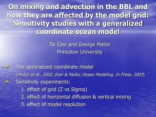
1. On mixing and advection in the BBL and how they are affected by the model grid: Sensitivity studies with a generalized coordinate ocean model Tal Ezer and George Mellor Princeton University The generalized coordinate model (Mellor et al., 2002; Ezer & Mellor, Ocean Modeling, In Press, 2003) Sensitivity experiments: 1. effect of grid (Z vs Sigma) 2. effect of horizontal diffusion & vertical mixing 3. effect of model resolution

2. The generalized coordinate system Z(x,y,t)=(x,y,t)+s(x,y,k,t) ; 1<k<kb, 0<<-1 Special cases Z-level: s=(k)[Hmax+ (x,y,t)] Sigma coord.: s=(k)[H(x,y)+ (x,y,t)] S-coordinates (Song & Haidvogel, 1994): s=(1-b) func[sinh(a,)]+b func[tanh(a,)] a, b= stretching parameters Other adaptable grids Semi-isopycnal?: s=func[(x,y,z,t)]

3. Potential Grids

4. Effect of model vertical grid on large-scale, climate simulations Experiments: • Start with T=T(z) • Apply heating in low latitudes and cooling in high latitudes • Integrate model for 100 years using different grids (all use M-Y mixing)

6. The problem of BBLs & deep water formation in z-level models is well known (Gerdes, 1993; Winton et al., 1998; Gnanadesikan, 1999) I-1 I I+1 • Some Solutions: • Embedded BBL • (Beckman & Doscher, 1997; • Killworth & Edwards, 1999; • Song & Chao, 2000) • “Shaved” or partial cells • (Pacanowski & Gnanadesikan, 1998; • Adcroft et al., 1997) K-1 K K+1 T T U W T

7. Dynamics of Overflow Mixing & Entrainment (DOME) project Bottom Topography Initial Temperature(top view) (side view) embayment slope deep

8. Simulation of bottom plume with a sigma coordinate ocean model (10km grid)

10. The effect of horizontal diffusivity on the Sigma coordinate model(tracer concentration in bottom layer)

11. DIF=10 DIF=100 DIF=1000 10 days 20 days

12. The effect of grid type- Sigma vs. Z-level coordinates

13. ZLV-10 days SIG-10 days ZLV-20 days SIG-20 days

14. Increasing hor. diffusion causes thinner BBL in sigma grid but thicker BBL in z-level grid! SIG DIF=10 SIG DIF=1000 ZLV DIF=10 ZLV DIF=1000

15. The BBL: More stably stratified & thinner in SIG Larger downslope vel. in SIG, but much larger (M-Y) mixing coeff. in ZLV

16. The difference in mixing mechanism:SIG is dominated by downslope advection, the ZLV by vertical mixing

17. The effect of grid resolution or Is there a convergence of the z-lev. model to the sigma model solution when grid is refined? The Problem: to resolve the slope the z-lev. grid requires higher resolution for both, horizontal and vertical grid. New high-res. z-grid experiment: quadruple hor. res., double ver. res.

18. 10 km grid 2.5 km grid

19. Increasing resolution in the z-lev. grid resulted in thinner BBL and larger downslope extension of the plume. ZLV: 10 km, 50 levels ZLV: 2.5 km, 90 levels

20. The thickness of the BBL and the extension of the plume are comparable to much coarse res. sigma grid. SIG: 10 km, 10 levels ZLV: 2.5 km, 90 levels

21. How do model results compare with observations? Density section along the plume Thickness across the plume From: Girton & Sanford, Descent and modification of the overflow plume in the Denmark Strait, JPO, 2003

23. Comments: • Terrain-following grids are ideal for BBL and dense overflow problems. (Isopicnal models are also useful for overflow problems, but may have difficulties in coastal, well mixed regions) • Hybrid or generalized coordinate models may be useful for intercomparison studies, or for optimizing large range of scales or processes in a single code. • However, how to best construct such models and how to optimizing such grids for various applications are open questions that need further research.