Download

1 / 58
580 likes | 677 Views
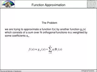
Data Driven Function Approximation. One link. Given X t what is the joint angle P. Y. x t. P. x. Plot1d. Plot a function that maps joint angle P to tool position X t. clear all fstr=input('input a function: x.^2+cos(x) :','s'); fx=inline(fstr); range=2*pi; x=linspace(-range,range);

E N D
One link Given Xt what is the joint angle P Y xt P x
Plot1d Plot a function that maps joint angle P to tool position Xt clear all fstr=input('input a function: x.^2+cos(x) :','s'); fx=inline(fstr); range=2*pi; x=linspace(-range,range); y=fx(x); max_y=max(abs(y)); plot(x,y/max_y); hold on;
Black box Black box Xt P range=2*pi; linspace(-range,range); observation N=input('keyin sample size:'); x=rand(1,N)*2*range-range; n=rand(1,N)*0.1-0.05; y=fx(x)/max_y+n; figure plot(x,y,'.');
Adaptive function Desired output Network output Input error
Network function Weight sum of hyper-tangent functions
Network b1 tanh r1 b2 1 a1 tanh r2 a2 x ……. bM rM aM tanh rM+1 1
Procedure 1: MLP evaluation • Input r,a,b and x,M • y=r(M+1) • Set M to the length of a • For m=1:M • Add r(i)*tanh(x*a(i)+b(i)) to y • Return y
Matlab code eval_MLP.m function y=eval_MLP(x,r,a,b,M) y=r(M+1); for m=1:M y=y+r(m)*tanh(x.*a(m)+b(m)); end return
Mean square error Given Find to minimize
Procedure 2: Mean square error • Input x,y,a,b,r • Set E to zero • Set n to the length of x • For i=1:n • Calculate the square error of approximating y(i) by f(x;r,a,b) • Add the error to E • Return E
Matlab code mean_square_error2.m function E=mean_square_error2(x,y,a,b,r) E=0; M=length(a); n=length(x); for i=1:n s_err=(y(i)-eval_MLP(x(i),r,a,b,M)).^2; E=E+s_err; end E=E/n; return
Desired output Network output Input error Application Black box plot1d.m Xt P observation Create paired data sampling.m Leaning learning.m
Matlab code Function approximation for an arbitrary target function fa1d.m
Y xt P x Inverse kinematics
Construction of inverse kinematics • Procedure • Input a 1d forward kinematics • Sampling to form paired data • Input-output swapping • Rescaling • Learning
Data preparation Black box plot1d.m Xt P observation Create paired data sampling.m Rescaling temp=x; x=y; y=temp; swapping max_y=max(y); y=y/max_y; plot(x,y,'.')
Learning inverse kinematics Desired output Network output Input error Leaning learning.m
Matlab code fa1d_inv.m MSE for training data 0.336461 ME for training data 0.490247 Unacceptable training errors
Multiple outputs • Inverse kinematics • Conflicts of I/O relation • Two distinct outcomes for the same input
First order derivative • Forward kinematics should be characterized by two outputs for construction of inverse kinematics Two observations Xt Black box plot1d.m P Derivative
Symbolic differentiation demo_diff.m function demo_diff() % input a string to specify a function % plot its derivative ss=input('function of x:','s'); fx=inline(ss); x=sym('x'); ss=['diff(' ss ')']; ss1=eval([sprintf(ss)]); fx1=inline(ss1) x=linspace(-pi,pi); plot(x,fx(x),'b');hold on; plot(x,fx1(x),'r'); return
Data preparation Two observations Xt Black box plot1dd.m P Dt Derivative
Reverse kinematics Xt Reverse Kinematics P Dt Derivative plot3(y1,y2,ix)
Segmentation • Procedure • Input paired data,(x,y) • Sort data by y
Write a matlab function to divide paired data to four segments
Two links (xt yt) Y P2 P1 x
Learning forward kinematics learn_MLP.m eval_MLP2.m fa2d.m
Inverse kinematics At the position level, the problem is stated as, "Given the desired position of the robot's hand, what must be the angles at all of the robots joints? "
Exercise • Write matlab functions to implement forward and inverse kinematics of a two-link robot
Example l1=1;l2=1; p1=pi/3;p2=pi/5; [x,y]=fkin(p1,p2,l1,l2) [p1,p2]=inverse_kin(x,y,l1,l2); p1/pi p2/pi
x=linspace(-2,2); plot(x,x); hold on; plot(x,sqrt(4-x.^2)) plot(x,-sqrt(4-x.^2))
function F = myfun(x) F(1) = x(1).^2 + x(2)^2-4; F(2) = x(1) - x(2); return