Download
1 / 22
220 likes | 228 Views
Zeta Zero Pair Correlation. Zeros of zeta function have real part 0.5 (Reimann’s hypothesis, called the critical line) number of the nth zeta zero is of the form z(n)=0.5 + i. t(n) where t(n) is called the height of the nth zero

E N D
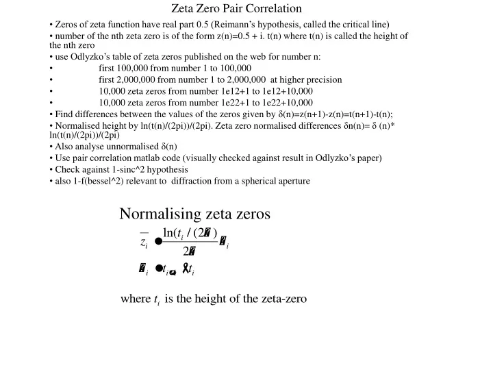
Zeta Zero Pair Correlation Zeros of zeta function have real part 0.5 (Reimann’s hypothesis, called the critical line) number of the nth zeta zero is of the form z(n)=0.5 + i. t(n) where t(n) is called the height of the nth zero use Odlyzko’s table of zeta zeros published on the web for number n: first 100,000 from number 1 to 100,000 first 2,000,000 from number 1 to 2,000,000 at higher precision 10,000 zeta zeros from number 1e12+1 to 1e12+10,000 10,000 zeta zeros from number 1e22+1 to 1e22+10,000 Find differences between the values of the zeros given by δ(n)=z(n+1)-z(n)=t(n+1)-t(n); Normalised height by ln(t(n)/(2pi))/(2pi). Zeta zero normalised differences δn(n)= δ (n)* ln(t(n)/(2pi))/(2pi) Also analyse unnormalised δ(n) Use pair correlation matlab code (visually checked against result in Odlyzko’s paper) Check against 1-sinc^2 hypothesis also 1-f(bessel^2) relevant to diffraction from a spherical aperture Normalising zeta zeros
Montgomery’s Pair Correlation Conjecture 1973 The normalised zeta zero differences hypothesed to have a pair correlation of (1-sinc^2) which is also associated with the pair correlation of eigenvalues of a random Hermitian matrix (a Gaussian Unitary Ensemble, GUE) My hypothesis (1-sinc^2) is also associated with wave diffraction from a square aperture, whose shape depends on the phase of the distribution. The (1-sinc^2) is the plane-wave phase shape (the far-field, i.e I’m hypothesising at greater heights up the critical line). Closer in (i.e at lower heights) the shape changes as the phase becomes more circular and the Fresnel function comes into play. I want to check the pair correlation shapes here to see if this could be so. Pair correlation function
Pair Correlation Function My Matlab Code Define number of bins in range required: following Odlyzko= 0 to 3 in steps of 0.05 (1/20). Number of elements to add. Doesn’t make any difference to result if i larger than, say, 1000 x is the vector of normalised zeta zero differences Filter function adds a number of elements together. The number is given by the vector ‘add’. e.g x=[1,2,3,4,5,6] add=[1], adds one element xsum=filter([1],1,x)=[1,2,3,4,5] add=[1 1], adds two elements xsum=filter([1 1],1,x)=[3,5,7,9,11] etc For each loop find number of differences that are in each bin from 0 to 3 in 0.05 steps using histogram For each loop find cumulative sum of number of differences that are in each bin from 0 to 3 in 0.05 steps using histogram Increase the size of ‘add’ i.e number of differences to add together for each loop e.g [1],[1 1], [1 1 1] etc up to [1000 1’s].
Pair Correlations from my Matlab Code Compared to Odlyzko Result from Odlyzko’s paper First 100,000 for comparison Dots are first 100,000 from my Matlab code along with 1-sinc^2(x)
Pair Correlations from my Matlab Code Second 50,000 First 50,000
Pair Correlations from my Matlab Code First 500,000 Second 500,000
Pair Correlations from my Matlab Code Third 500,000 Fourth 500,000
Pair Correlations from my Matlab Code First 2,000,000 normalised zeta zeros, pair correlation plotted every 100,000 (20 plots overlaid). Also plotted is 1-sin^2 and Airy function in green so doesn’t look like an Airy function
Pair Correlations from my Matlab Code First 2,000,000 normalised zeta zeros. Also plotted is 1-sinc^2.
Pair Correlations from my Matlab Code 10,000 Zeta Zeros starting from Numbers 10^12 +1 to 1-^12+1000 up to 10^22+1 to 10^22+10000 10^12+1 to 10^12+10,000 10^22+1 to 10^22+10,000
Pair Correlations from Gourdon Two billion normalised zeta zeros differences. N=10^13+1 through 10^13+2e9. Bin size 0.01. Also plotted is 1-sinc^2. (Data from Gourdon)
Pair Correlations from Gourdon Two billion normalised zeta zeros differences. N=10^14+1 through 10^14+2e9. Bin size 0.01. Also plotted is 1-sinc^2. (Data from Gourdon)
Pair Correlations from Gourdon Two billion normalised zeta zeros differences. N=10^15+1 through 10^15+2e9. Bin size 0.01. Also plotted is 1-sinc^2. (From Gourdon)
Gourdon has data to 10^24 but can’t see much difference so look at differences from 1-sinc^2 for the various zeta zero numbers. So Gourdan look at differences between probability density function (pdf) of the normalised zeta zero spacing and the GUE pdf shown next slide.
Differences between pair spacing probability density and GUE from Gourdon • becomes MORE like GUE as increase in height up the critical line Difference
But I will look at differences between the pair correlation (blue dots) of the normalised zeta zero spacings and the GUE function of 1-sinc^2 (red curve) for 2 billion normalised zeta zeros from numbers N=10**13+1 to N=10**13+2e9 to N=10**24+1 to N=10**24+2e9 from Gourdans data Use Matlab code plot_gourdan_pair_correlation_gue_differences.m
Differences between the pair correlations of the normalised zeta zero spacings and the GUE function of 1-sinc^2 for 2 billion normalised zeta zeros from numbers N=10**13+1 to N=10**13+2e9 to N=10**24+1 to N=10**24+2e9 from Gourdan’s data • there seems to be a ‘transition’ region at spacing approx 0.7 • spacing 0.7 is a Pivot Point of unknown relevance • for spacing approx>0.7as go higher up the critical line pair correlation becomes MORE like GUE • for spacing approx<0.7as go higher up the critical line pair correlation becomes LESS like GUE • this is different to Gourdan’s differences of normalised spacing to pdf where the distribution becomes more like GUE for all spacings as increase height (from looking at previous Gourdan’s plot) • this extra difference by using the pair correlation will give an extra feature to decide between hypothesis to explain these difference effects. • there is a wave on the distribution with maximum peaks at approx zeta zero spacing of (0.2 going to 0.4 with height), 0.8, 1.8, 2.8, 3.8...the delta of the peaks seems to be 1. Observations note: small y scale +/-0.006 Black dots are zeta zeros for N=10**13+1 to 10**13+2e9 Blue dots are zeta zeros for N=10**24+1 to 10**24+2e9 Pivot point 0.7
Pair Correlations from my matlab code Unormalised zeta zero data
Pair Correlations from my Matlab Code First 100,000
Pair Correlations from my Matlab Code First 500,000 Second 500,000
Pair Correlations from my Matlab Code Fourth 500,000 Third 500,000
But I will look at differences between the pair correlation (blue dots) of the normalised zeta zero spacings and 1-sinc for 2 billion normalised zeta zeros from numbers N=10**13+1 to N=10**13+2e9 to N=10**24+1 to N=10**24+2e9 from Gourdans data Use Matlab code plot_gourdan_pair_correlation_1_minus_sinc_differences.m all overlay and note: larger y axis +/- 0.3. Not a sensitive measure of differences with height up critical line