Download
1 / 48
480 likes | 485 Views
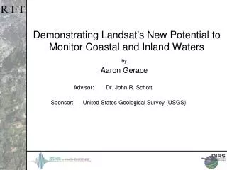
Demonstrating Landsat's New Potential to Monitor Coastal and Inland Waters. by Aaron Gerace Advisor: Dr. John R. Schott Sponsor: United States Geological Survey (USGS). Research Motivation. Desire to monitor the Earth’s coastal and fresh water supply.

E N D
Demonstrating Landsat's New Potential to Monitor Coastal and Inland Waters by Aaron Gerace Advisor: Dr. John R. Schott Sponsor: United States Geological Survey (USGS)
Research Motivation • Desire to monitor the Earth’s coastal and fresh water supply. • No environmental satellite to date has the necessary characteristics… • High spatial resolution. • High radiometric fidelity. • Repeat Coverage. • Data are readily accessible. Rochester Embayment MODIS Rochester Embayment Landsat
Monitoring Fresh and Coastal Waters • Spatial Resolution: • Repeat Coverage: • Accessible Data 46 vs. 68 units of chlorophyll • Radiometric Fidelity: Significant changes in constituent concentrations often lead to small changes in water-leaving reflectance.
Monitoring Fresh Waters • Case 2 Waters: • Inland and coastal waters. • Optically complex case 2 waters contain significant levels of... • Chlorophyll-a • phytoplankton • Suspended Materials • runoff • Colored dissolved organic matter (CDOM) • Decaying organic matter • Issues: • Determine condition of water through constituent retrieval process. • Trophic status and trends • Characterize sedimentation in river plumes. • Predict beach closings. • Impact of sediment on the surrounding environment.
Overview of Research • Demonstrate that Landsat’s new OLI sensor is suitable for studying optically complex case 2 waters. • Radiometric fidelity. 1 46 vs. 68 units of chlorophyll Landsat 5: July 13th, 2009
Overview of Research 2. Develop an over-water atmospheric compensation algorithm for the OLI sensor. • OLI does not have the appropriate spectral coverage to utilize traditional water-based algorithms. Atmospheric Compensation 2
Objective 1: Model the improved features of the OLI sensor and demonstrate its improved radiometric fidelity. Landsat 5: July 13th, 2009
OLI Features: Enhanced Spectral Coverage ETM+ Response OLI Response
OLI Features: Quantization ETM+ (8-bit) OLI (12-bit)
ETM+ OLI OLI Features: Signal to Noise • About a factor of 5 improvement in SNR.
Modeling the Constituent Retrieval Process: Hydrolight Solar location Sensor location x 2000 Wind Speed CDOM CHL SM • Water IOPs • Absorb • Scatter
Modeling the Constituent Retrieval Process: At the Sensor Add Noise Resample Quantize AVIRIS ETM+ OLI
Modeling the Constituent Retrieval Process: CRA Top of Atmosphere Air/Water Interface CHL=3 SM=4 CDOM=7 CDOM SM CHL
Modeling the Constituent Retrieval Process: Summary Add Noise Resample Quantize CRA AVIRIS ETM+ OLI • Average residuals can be expressed as a percent of the total range of constituents. CHL [0 – 68], SM [0 – 24], CDOM [0 – 14] • 10% error is our target for this experiment.
Objective 2: Atmospheric Compensation Develop an over-water atmospheric compensation algorithm specifically for the OLI sensor.
OLI ApproachCase 2 Waters • Purpose: Convert TOA radiances to water-leaving reflectances. • Issue: OLI doesn’t have 2 NIR bands which are required by traditional water-based algorithms. • Gordon’s method (SeaWiFS). • 2 methods developed: • Blue Band method. • NIR/SWIR band ratio method.
OLI ApproachCase 2 Waters Water Atmosphere Water Atmosphere Image
OLI ApproachCase 2 Waters Dark Water Atmosphere Dark Water Atmosphere Image
OLI ApproachCase 2 Waters • Incorporate dark water component into an atmospheric LUT. 10km 15km 20km Atmosphere Dark Water • Mid-latitude Summer profile. • May 20th, 1999. • Standard gases • Rural aerosols • Varied visibility between 5 and 60 kilometers. AVIRIS: May 20th, 1999
OLI ApproachCase 2 Waters • Incorporate dark water constant into an atmospheric LUT. 10km 15km 20km Atmosphere Dark Water AVIRIS: May 20th, 1999
OLI Atmospheric Compensation Experiment 1: Simulated Data • Use same 2000 water pixels described in first experiment. • Propagate to the top of 23 kilometer visibility modeled atmosphere. • Signals are then spectrally sampled to OLI, half margin noise is added, and quantization effects included. • Average darkest 5% of signals in band 5 to determine atmosphere (22.97km). • Chosen atmosphere removed spectrally from all modeled pixels.
OLI Atmospheric Compensation Experiment 1: Simulated Data • 15% is our target error when atmospheric effects are included. • A typical scene contains hundreds of thousands of water pixels!
OLI Atmospheric Compensation Experiment 2: Simulated Scene • Simulated Image from Landsat 5 data • Lake Ontario (Dark Water) ROI used to determine atmosphere. • Chosen atmosphere removed globally from image. • Constituent retrieval algorithm implemented for 6 ROIs. Landsat 5: May 16th, 1999 Simulated Image
OLI Atmospheric Compensation Experiment 2: Simulated Scene 46 vs. 68 units of chlorophyll
Ongoing • Develop tool to spatially sharpen TIRS data With OLI • Done • Use TIRS thermal data to calibrate flow field of hydrodynamic model. • Alge outpus surface temperature • Proof of concept complete • Use Landsat reflective data to calibrate color of hydrodynamic model. • ALGE outputs sediment profiles. • Initial tool under test • Continue to investigate OLI atmospheric compensation. • 3 band method, perhaps.
OLI Atmospheric Compensation Experiment 3: Real Data • AVIRIS data (May 20th,1999) spectrally sampled to OLI’s sensor response function. AVIRIS: May 20th, 1999 Simulated OLI Data: May 20th, 1999
OLI Atmospheric Compensation Experiment 3: Real Data • OLI atmospheric compensation method tested over Cranberry Pond and Long Pond. • Deglint image. • 200 darkest values in bands 5 and 6 were used to determine atmosphere. • Atmospheric effects removed and constituent retrieval process performed. • Empirical Line Method. Cranberry Pond “OLI” Data Long Pond
OLI Atmospheric Compensation Experiment 3: Real Data • Initial errors are discouraging. • For Cranberry pond, CDOM retrieval is over 20%. • For Long Pond, retrieval errors for 2 constituents are greater than 30%.
OLI Atmospheric Compensation Experiment 3: Real Data Compensated Data Retrieved Reflectances Expected Reflectances Cranberry Pond Long Pond Spectral Average: Long Pond ROI
OLI Atmospheric Compensation Experiment 3: Real Data • More reasonable errors obtained. • For Cranberry pond, only suspended materials is over 15% retrieval error. • For Long Pond, retrieval errors for all constituents are less than 15%.
OLI Atmospheric Compensation Experiment 3: Real Data Expected Reflectances Retrieved Reflectances: Bias Corrected Retrieved Reflectances: Biased Cranberry Pond Long Pond
Objective 3: Develop techniques that will enable Landsat data to be used to calibrate a hydrodynamic model. ALGE Hydrodynamic Model Landsat 5: July 13th, 2009
Hydrodynamic Modeling: Inputs • To model the Genesee River plume, ALGE requires information from the scene of interest… • Static: Land/Water, latitude/longitude, bathymetry, voxel size, DOY, etc. • Dynamic: Environmental Measurements (hourly) • River data (flow rate, initial temperature) • Surface data (Pier / Rochester airport) • Upper air (Bufkit model) Landsat 5: July 13th, 2009 Northeastern United States
Hydrodynamic Modeling: Inputs • To model the Genesee River plume, ALGE requires information from the scene of interest… • Nudging Vectors (hourly). • Whole lake simulation provides nudging vectors for small scale simulation. ALGE Hydrodynamic Model Lake Ontario simulation: Surface Currents Landsat 5: July 13th, 2009
Hydrodynamic Modeling: Outputs • To model the Genesee River plume, ALGE requires information from the scene of interest… • Land/Water, latitude/longitude, bathymetry, voxel size, DOY, etc. • Environmental Measurements (hourly) • River data (flow rate, initial temperature) • Surface data (Pier / Rochester airport) • Upper air (Bufkit model) • Nudging Vectors (hourly) ALGE Hydrodynamic Model Landsat 5: July 13th, 2009
Hydrodynamic Modeling: Outputs • To model the Genesee River plume, ALGE requires information from the scene of interest… • Land/Water, latitude/longitude, bathymetry, voxel size, DOY, etc. • Environmental Measurements (hourly) • River data (flow rate, initial temperature) • Surface data (Pier / Rochester airport) • Upper air (Bufkit model) • Nudging Vectors (hourly) ALGE Hydrodynamic Model Landsat 5: July 13th, 2009
Hydrodynamic Modeling: Steady State • Run ALGE until model reaches a steady state. • Satellite data will not match model data… • Inaccurate inputs. • Model error. July 13th, 2009 July 2nd, 2009 Start Model Stop Model Landsat 5: July 13th, 2009
Hydrodynamic Modeling: Calibration • 24 hours prior to obtaining satellite data, the model is stopped and a calibration LUT created • Vary environmental parameters (about their nominal values) that will affect a plume’s shape. July 13th, 2009 July 2nd, 2009 July 12th, 2009 … … 10 day ALGE run (steady state period) Start Model 1 day (calibration period) …
Hydrodynamic Modeling: Calibration • Develop a calibration LUT whose domain is made up of parameter variations and whose range is made up of ALGE runs.
Hydrodynamic Modeling: Calibration • Nonlinear, least-squares optimizer is used to search the LUT. • Landsat data must be registered and atmospherically compensated. • The point in space that provides the best match contains the model that best describes the state of the environment.
Hydrodynamic Modeling: Results • RMS-error of 0.28 Kelvin. Landsat 5: July 13th, 2009 Optimal Model
Conclusions • OLI exhibits enormous potential to be used for monitoring case 2 waters. • The ability of the OLI atmospheric compensation algorithms were successfully demonstrated on simulated data, a simulated image, and a real image. • The sensor must be well calibrated. • Adequate SNR must be achieved. • Techniques were developed which enable Landsat data to be used to calibrate a hydrodynamic model.
Acknowledgements • Dr. Schott • My Committee • Dr. Vodacek • Dr. Salvaggio • Dr. Messinger • Dr. Sciremammano • DIRS Staff • Cindy Schultz • Dr. Schott’s students • Mom & Dad • The Outlaws • Matt and Prudhvi • Trisha