Download
1 / 42
420 likes | 751 Views
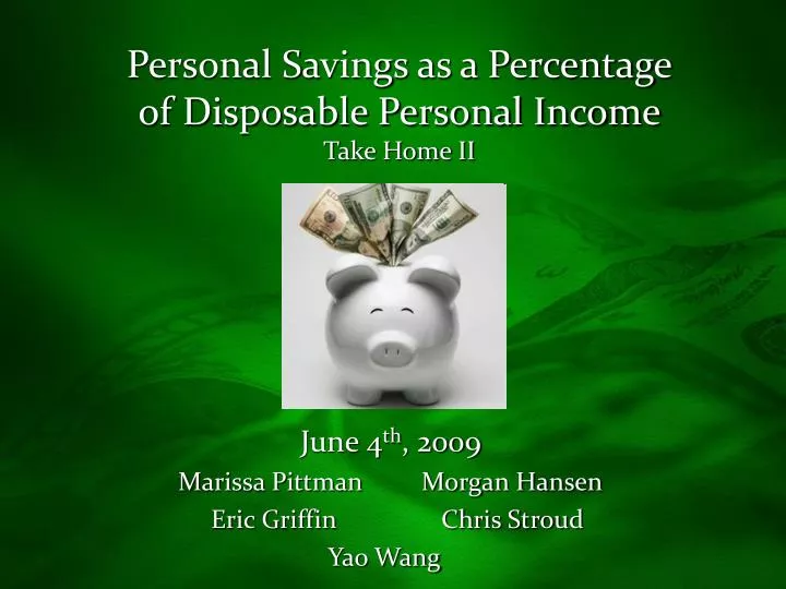
Personal Savings as a Percentage of Disposable Personal Income Take Home II. June 4 th , 2009 Marissa Pittman Morgan Hansen Eric Griffin Chris Stroud Yao Wang. Personal Savings

E N D
Personal Savings as a Percentageof Disposable Personal IncomeTake Home II June 4th, 2009 Marissa Pittman Morgan Hansen Eric Griffin Chris Stroud Yao Wang
Personal Savings The difference between household income (after taxes) and consumption expenditures. Negative number implies debt Positive number implies savings Personal Savings Household Income-Spending
As recently as April 2008, personal savings in the US totaled only 1.4 billion dollars In conjunction with the rapid collapse of the Economy in September 2008, personal savings has increased dramatically The latest number from April 2009 showed personal savings at $620.2 billion, the highest value in history. Personal Savings
Disposable Income Income (after taxes) that is available to you for saving or spending Disposable Income
Personal Savings (Semi-linear) Disposable Income (Exponential) Expected Results • Expect similar trends compared to the Personal Savings because decreasing and income is increasing
Why percentage and not net savings? Normalizes the data set Different people make different amounts of money It is safe to assume someone making $100,000/year will be saving more than someone making $30,000/year Savings as a Percentage of Disposable Income
This brings up our series, personal savings as a percentage of disposable income This ratio is also taken in order to account for inflation and the fact that incomes have been rising over time Savings/Income
Until the mid 1980s, people had been saving about 8-10 percent of their disposable income Starting in 1986 this number began trending downward due to easily obtainable credit (credit cards, lower mortgage rates, etc) Personal Savings as a Percentage of Disposable Personal Income
After the collapse of the economy in September this number began to shoot upward in conjunction with the increase in personal savings In April 2009 people were saving 5.7 percent of their disposable income which is the highest percentage since February 1995. Personal Savings as a Percentage of Disposable Personal Income
Appears to be random walk Hit peak in 1975 at 14.6% Has been steadily declining since Hit low in 2005 at -2.7% which meant people were spending more than they had Trace of Personal Savings as a Percentage of Disposable Personal Income
Multi-peaked Large Jarque-Bera statistics Further evidence the data set is random walk Histogram of Personal Savings as a Percentage of Disposable Personal Income
Correlogram of Personal Savings as a Percentage of Disposable Personal Income • The correlogram shows a slow decay in the autocorrelation • The PACF value at lag 1 is close to one • Both further indicators of a random walk
The unit root test returns a negative value that is not sufficiently more negative than the critical values Can’t reject null hypothesis The time series is not stationary. Unit Root Test of Personal Savings as a Percentage of Disposable Personal Income
The trace of the differenced values looks to be white noise The peaks indicate some periods of heightened variance. Differenced Trace of Personal Savings as a Percentage of Disposable Personal Income
The histogram of the differenced values is kurtotic It is single peaked which is a sign of stationarity but still not acceptable Differenced Histogram of Personal Savings as a Percentage of Disposable Personal Income
Differencing the time saving has removed the autocorrelation trends The PACF at lag 1 value is no longer close to 1 The spikes in PACF at lag 1 and lag 3 are evidence that an ARMA model of a AR(1) and AR(3) would be a good initial model estimation Differenced Correlogram of Personal Savings as a Percentage of Disposable Personal Income
The unit root test of the differenced series returns a negative value that is sufficiently more negative than the critical values Reject the null hypothesis Time series is stationary Dsaving does not contain a unit root. Differenced Unit Root Test of Personal Savings as a Percentage of Disposable Personal Income
ARMA Model 1 returns significant t-stats on both terms. AR(1)=-7.28 AR(3)=-4.46 ARMA Model 1 • The constant is not significant • C=-0.23
The ARMA terms have removed the PACF spikes at lags 1 and 3 but the Q stats are still high. The spike at lag 2 may be eliminated with a MA(2). Correlogram of ARMA Model 1
ARMA Model 2 returns significant t-stats on all 3 terms. AR(1)=-8.97 AR(3)=-4.43 MA(2)=-6.04 The constant is not significant C=-0.37 Durbin-Watson statistic is approximately 2.0, indicating no serial correlation ARMA Model 2
All spikes have now been eliminated and Q-stats are now low L looks orthogonal, with fairly low Q-statistics and high probabilities Model has now proven to be stationary and an accurate estimation Correlogram of ARMA Model 2
The low F-statistic also confirms that there’s no serial correlation. Probability is less than critical at 0.28 Serial Correlation Test of Model 2
The residuals are orthogonal Tracking the actual trace well Peaks still implicated heightened variance Actual, Fitted and Residual Plot of Model 2
The residuals are still single peaked Although highly kurtotic with afat tail Could suggest existence of conditional heteroskedasticity Histogram of Residuals for Model 2
The episodic variance shows some spikes This indicates that residuals are not homoskedastic Heteroskedasticity is present Trace of Squared Residuals for Model 2
The correlogram of squared residuals shows high Q-statistics There are some significant lags Correlogram of Squared Residuals for Model 2
The F-statistic is significant enough to reject the null hypothesis of homoskedasticity Consistent with former evidences Heteroskedasticity exists ARCH Test of Model 2
Added ARCH GARCH to account for heteroskedasticty of the residuals Z-statistics of coefficients showed the model to be significant ARCH GARCH Estimation of Model 2
Correlogram is orthogonal Lower Q-stats were achieved Probabilities are above 0.05 ARCH GARCH Correlogram for Model 2
The residuals are orthogonal Tracking the actual trace well Still some variance but tracking is better GARCH Actual, Fitted, and Residual Plot for Model 2
Histogram is single peaked Kurtosis is still an issue but all other problems are resolved Histogram of Standardized Residuals for Model 2
Estimate of h(t) by making GARCH variance series Trace of GARCH for Model 2
The F-statistic now is not significant to reject the null hypothesis of homoskedasticity The model we estimated above seems to be a good fit Heteroskedasticity no longer exists ARCH GARCH Test for Model 2
In sample forecast to test for accuracy Forecast of Model 2Non-recolored
In sample variance Variance is increasing over time Leveling off Forecast of Variance for Model 2
Recession causing shocks to data set People would continue to spend at high rates or save at low rates Forecast of Model 2 In Sample
As said before there is an increase in saving due to our recent recession Purpose of the project is to answer is if people will continue to save as the economy comes out of the recession Project Purpose
Out of sample forecast for the next year Forecast for Model 2Non-recolored
Out of sample variance Variance is decreasing over time Leveling off Forecast of Variance for Model 2
Stops going up and steadies Current trend of rising is going to cease Out of Sample Forecast for Model 2
The results of our forecast indicate that in fact people will continue to save as the recession subsides This makes sense intuitively because credit conditions will remain tighter People will need to save more for larger down-payments on homes, cars, and other loans that are now required due to more stringent loan requirements. Final Results