Download
1 / 25
250 likes | 262 Views
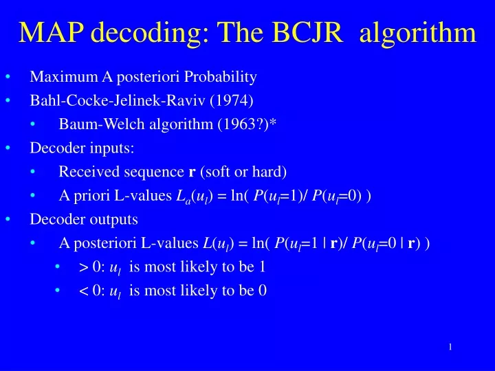
MAP decoding: The BCJR algorithm. Maximum A posteriori Probability Bahl-Cocke-Jelinek-Raviv (1974) Baum-Welch algorithm (1963?)* Decoder inputs: Received sequence r (soft or hard) A priori L-values L a ( u l ) = ln( P ( u l =1)/ P ( u l =0) ) Decoder outputs

E N D
MAP decoding: The BCJR algorithm • Maximum A posteriori Probability • Bahl-Cocke-Jelinek-Raviv (1974) • Baum-Welch algorithm (1963?)* • Decoder inputs: • Received sequence r (soft or hard) • A priori L-values La(ul) = ln( P(ul=1)/ P(ul=0) ) • Decoder outputs • A posteriori L-values L(ul) = ln( P(ul=1 | r)/ P(ul=0 | r) ) • > 0: ul is most likely to be 1 • < 0: ul is most likely to be 0
BCJR (Continued) AWGN
MAP algorithm • Initialize Forward recursion 0(s) and backward recursion N(s) • Compute branch metrics {l(s’,s)} • Carry out forward recursion {l+1(s)} based on {l(s)} • Carry out backward recursion {l-1(s)} based on {l(s)} • Compute APP L-values • Complexity: approximately 3xViterbi • Requires detailed knowledge of SNR • Viterbi just maximizes rv, does not require exact SNR
BCJR (Continued) Information bits Termination bits
Log-MAP algorithm • Initialize Forward recursion 0*(s) and backward recursion N*(s) • Compute branch metrics {l*(s,s’)} • Carry out forward recursion {l+1*(s)} based on {l*(s)} • Carry out backward recursion {l-1*(s)} based on {l*(s)} • Compute APP L-values • Advantages over MAP algorithm: • Easier to implement • Numerically stable
Max-log-MAP algorithm • Replace max* by max: delete table lookup correction term • Advantage: Simpler, faster (?) • Forward and backward pass equivalent to Viterbi decoder • Disadvantage: Less accurate (but the correction term is limited in size by ln 2)
Example: log-MAP 0,44 3,06 0,45 1,60 3,02 -0,75 +1,45 +0,25 -0,35 +0,75 -1,45 +0,45 1,60 0 1,59 1.34 -0,45 3,44 0 -0,45 +0,35 -0,25 +0.48 +0.62 -1,02 0 0 • Assume Es/N0=1/4 = - 6.02 dB • R=3/8 so Eb/N0=2/3 = - 1.76dB
Example: Max-log-MAP 0,45 2,34 3,05 1,60 -0,20 -0,75 +1,45 -0,35 +0,25 +0,75 -1,45 1,60 +0,45 0 1.20 3,31 -0,45 1,25 0 -0,45 +0,35 -0,25 -0,07 +0,10 -0,40 0 0 • Assume Es/N0=1/4 = - 6.02 dB • R=3/8 so Eb/N0=2/3 = - 1.76dB
Punctured convolutional codes • Recall that an (n,k) convolutional code has a decoder trellis with 2k branches going into each state • More complex decoding • Solutions • Syndrome decoding • Bit-oriented trellis • Punctured codes • Start with low-rate convolutional mother code (rate 1/n?) • Puncture (delete) some code bits according to predetermined pattern • Punctured bits are not transmitted. Hence the code rate is increased, but the distance between codewords is reduced • Decoder inserts dummy bits with neutral metrics contribution
Example: Rate 2/3 punctured from rate 1/2 dfree = 3 • The punctured code is also a convolutional code • Note the bit-level trellis
More on punctured convolutional codes • Rate compatible punctured convolutional codes • For applications that needs to support several code rates • For example adaptive coding • Sequence of codes obtained by repeated puncturing • Advantage: One decoder can decode all codes in family • Disadvantage: Resulting codes may be sub-optimum • Puncturing patterns • Usually periodic puncturing maps • Found by computer search • Care must be exercised to avoid catastrophic encoders
Best punctured codes 7 5 10 1 !4 2 5 3 6 6 27 7 17
Tailbiting convolutional codes • Purpose: Avoid the terminating tail (rate loss) • without distance loss? • Cannot avoid distance loss completely • Tailbiting codes: Paths through trellis • Codewords can start in any state • Gives 2as many codewords • But each codeword must end in the same state that it started from • …Gives 2-as many codewords • Tailbiting codes increasingly popular for moderate length purposes • DVB: Turbo codes with tailbiting component codes
”Circular” trellis • Decoding • Try all possible starting states (multiplies complexity by 2) • Suboptimum Viterbi: Let decoding proceed until best ending state found, continue ”one round” from there • MAP: Similar
Example: Feedforward encoder Feedforward: always possible to find an information vector that ends in the proper state-> can start in any state and end in any state
Example: Feedback encoder • Feedback encoder: Not always possible, for every length, to construct a tailbiting systematic recursive encoder • For each u: must find unique starting state • L*=6 not OK • L*=5 OK
Tailbiting codes as block codes • Tailbiting codes are block codes
Suggested exercises • 12.27-12.39