Download
1 / 45
450 likes | 573 Views
Formation of Massive Galaxies. T.Naab , P. Johansson, R. Cen, K . Nagamine , R. Joung and J.P.O. Princeton , 28 Sept 2010. The Questions ?.

E N D
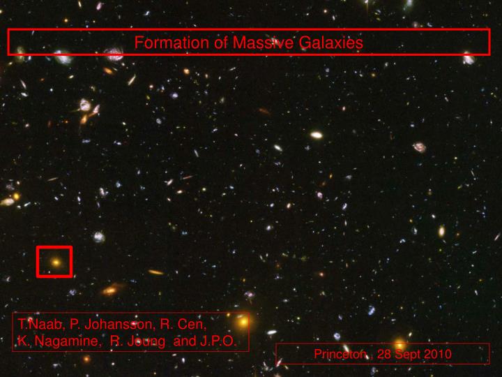
Formation of Massive Galaxies T.Naab, P. Johansson, R. Cen, K. Nagamine, R. Joungand J.P.O. Princeton , 28 Sept 2010
The Questions ? Can we start with initial conditions taken from the now standard model of cosmology, add standard physics, compute forwards and end with galaxies like those we see about us? Predictive and falsifiable. It could fail! [Unlike the “semi-analytic” method] What ingredients in physics are essential? Focus on massive galactic systems – giant ellipticals.
Focus: High Resolution Simulation of Massive Galaxy Formation ApJ.L.,658,710 (2007) ApJ.,697, 38 (2009) ApJ.L.,699,L178 (2009)
But first, what have we learned from 50 years of observations? • Giant elliptical galaxies form early and grow in size and mass without much late star-formation. • Major mergers are uncommon at late times (or else disk galaxies would have been destroyed). • Dark matter does not dominate the inner parts of elliptical galaxies. • Half of all metals are ejected from massive systems (cf winds and cluster metals).
NB, fluctuation level only 10-5 at high redshift Cosmological Simulation:Start with WMAP CBR Sky Hinshaw et al; 2008
WMAP Spectrum of Cosmic Perturbations (Amplitude)2 (Aplitude)2 Spherical Harmonic
In Detail: Best Current Cosmological Model (prior: LCDM) • tot= 1, ~flat geometry [obs =1.010 +0.016] • cdm= 0.22 ± 0.02 • baryon= 0.044 ± 0.002 • lambda= 0.73 ± 0.03 • n = 0.962 ± 0.015 • H0 = 71.5 ± 1.5 km/s/Mpc • 8 = 0.80 ± 0.01 • scat=0.086 ± 0.002 Tegmark et al (SDSS, 2005); Spergel et al (WMAP5, 2008) Ignore the details! Note that there are four components and small errors.
How to compute cosmic structure formation?(cartoon version) Recombination Nucleosynthesis linear perturbation theory nonlinear simulations
Computing the Universe: locally, growth of perturbations computed classically; numerical hydro required to reach the current epoch • Transformation to co-moving coordinates x=r/a(t) • Co-moving cube, periodic boundary conditions • Lbox >>lnl Lbox
Methods • Particle methods. Put down particles and move according to forces. Now at ~ 10003 for DM and ~ 5003 for “smooth particle hydrodynamics” particles. • Use fixed mesh. Very efficient ~ 20003 • Use adaptive mesh refinement: AMR with four levels each a factor of 8 in mass. • Use structured mesh.
First Step: Evolution of Dark Matter Component • Put down particles on a grid ( ~ 10^9 particles) with slight perturbations of the positions consistent with the early large scale structure given by CBR. • Give them small velocities consistent with the density structure and the continuity equation. • Calculate the accelerations of all the particles from Newton’s laws (in principle a calculation of order N*(N-1)/2). But algorithms are used which are N*log(N). • Advance positions and velocities given the velocities and accelerations to find the new distribution of particles. • Go back to step (3) and iterate to find the evolution of structure.
fast forward to structure growth computed in dark matter component ->
Second Step: hydrodynamic treatment of one piece. • Select region of interest. • Put down finer grid. • Add hydrodynamic equations. • Add atomic physics: adiabatic, + cooling, +heating, + non-equilibrium ionization. • Radiative transfer: global average, +shielding of sinks, +distribution of sources. • Heuristic treatment of star-formation. • Repeat calculation using tidal forces from larger region and do details of smaller region.
What have we learned? • The onset of galaxy formation is early and follows re-ionization at z = 6. High sigma peaks rapidly form stars from merging streams to initiate formation of cores of most galaxies. Disks and massive envelopes are formed later.
What is the observational* evidence (M. Kriek; ‘09) z ~ 2.5 *Chart color represents specific star formation rate: high rate = blue.
Detailed Hydro Simulations (N,J,O&E : 2007, ApJ, 658,710) Convergence to low and to a flat rotation curve at high resolution:
In Situ Star Formation Convergence to stellar system formed very early which quickly becomes “red and dead”.
Questions • Convergence: how do results change with resolution improvement; and why was high resolution needed? • Why does gas temperature increase though cooling time is short and no feedback was included? • Why is there a dramatic evolution of size? • Why is galaxy “red and dead” early but continues to grow in luminosity? ANSWER: TWO PHASE GROWTH WITH LARGE GRAVITATIONAL HEATING IN THE SECOND PHASE.
Gas Properties Gas, at all radii, becomes hotter with time despite fact that the “cooling time”< the Hubble time! Why?
2) Physics - why does gas not cool? • Gas is steadily being heated by in-falling new gas ( -PdV and Tds). • “Dynamical Friction” due to in-falling stellar lumps is very important for evolution of the stellar and DM components. • Of course “feedback” from central black holes and from supernovae also exists and must be complementary to effects listed above (and this is now being added to the codes – thesis projects).
20100929_Ostriker.mpg is not embedded in the presentation. Can be viewed separately or linked.
Half-Light Radii of In-situ and Accreted Stars A Normal Elliptical: fits Sersic Profile (detailed kinematics ok as well)
Astronomy • Two phase growth. First, in-situ star-formation from in-falling cold gas, and then accretion of stellar lumps. • DM initially increases in density (adiabatic contraction) and then decreases (dynamical friction). • Metal rich component in center from in-situ star-formation and metal poor component in outskirts due to stellar in-fall of old and small systems. • Stellar system grows in size with time and central velocity dispersion actually declines with time
Size evolution - substantial growth (observed and computed); what is the cause?
First attempt at showing data from 100^3 simulation (L.Oser)
Assembly of galaxies: Stellar material from minor mergers is made at early times and added at late times.
Binding Energy ~ 1060 erg from both in-situ and accreted stars: - In-situ energy is radiated, - Accreted energy heats gas and pushes out DM
(B-E)/s~ 1042.5 erg/s from both in-situ and accreted stars: - In-situ energy is radiated, - Accreted energy heats gas and pushes out DM.
What have we learned? Old news. • For massive systems the 1977 work of Binney, Silk and Rees & Ostriker appears to be correct : Cooling time of gas becomes longer than the dynamical time and star formation ceases. Systems live in hot bubbles and then grow by accretion of smaller stellar systems.
3) Why is there a dramatic evolution of size?4) Why is galaxy “red and dead” early but continues to grow in luminosity? • Evolution of size is apparent, not real. Both components keep roughly constant in size, but mean size grows as accreted material dominates. • During the second phase, the luminosity and stellar mass may double but very few stars are formed.
Simplest Physical Modeling - via Virial Theorem • Make initial, stellar system dissipatively from cold gas with gr radius RI, Mass MI, velocity dispersion < VI2>& energy EI: • EI = - 0.5 G MI2 / RI = -0.5 MI < VI2> • Add stellar systems conserving energy with total Mass MA = MI, velocity dispersion < VA2>= < VI2>& energy EA: • EA = -0.5 MI < VI2>
To make combined stellar system with grav radius RF, Mass MF = MI(1 + ), velocity dispersion < VF2>& energy EF: • EF = - 0.5 G MF2 / RF = -0.5 MI < VF2>(1+ ) • Then, equating total initial and final states • EF = EI + EA, gives for the ratios of the in-situ to the ultimate state as follows: • (< VF2>/ < VI2>) =[ (1 + ) / ( 1 + ) ] • (RF /RI ) = [ (1 + )2 / ( 1 + ) ] • (F/ I)= [ (1 + )2 / ( 1 + )3 ]
If the “accretion” consists of “major mergers”, with mass ratio unity, then is also unity and the above formulae reduce to the classic result, BUT If the added systems have much lower velocity dispersions than the original system, then << 1,and the velocity dispersion declines, with the surface density declining dramatically, as in the numerical simulations.
Conclusions: High Mass Systems • High resolution SPH simulations without feedback produce normal, massive but small elliptical galaxies at early epochs from in-situ stars made from cold gas. • Accreted smaller systems add, over long times, a lower metallicity stellar envelope of debris (obvious test exists). • The physical basis for the cutoff of star-formation is gravitational energy release of in-falling matter acting through -PdV and +Tds energy input to the gas. • This simple two phase process explains the decline in velocity dispersion and surface brightness at later times. • Feedback from SN and AGN are real phenomena - but secondary and mainly important for clearing out gas at late times and reducing stellar mass as compared to the simulations.
To Be Done • Do many more cases at high resolution; and repeat with different codes. • Look at X-ray properties.☐ • Improve gas cooling and radiative transfer.☐ • Repeat with SNI&II and AGN feedback.☐ • Add recycled gas.☐ (and make more mpgs!)