Download
1 / 41
410 likes | 629 Views
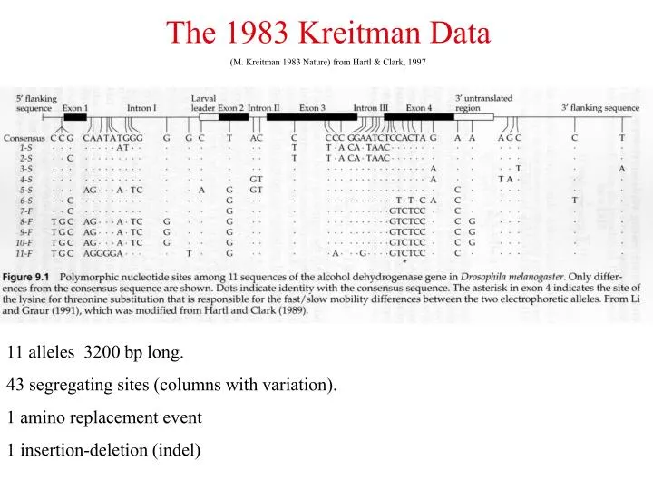
The 1983 Kreitman Data (M. Kreitman 1983 Nature) from Hartl & Clark, 1997. 11 alleles 3200 bp long. 43 segregating sites (columns with variation). 1 amino replacement event 1 insertion-deletion (indel). Coalescent Theory in Biology

E N D
The 1983 Kreitman Data (M. Kreitman 1983 Nature) from Hartl & Clark, 1997 11 alleles 3200 bp long. 43 segregating sites (columns with variation). 1 amino replacement event 1 insertion-deletion (indel)
Coalescent Theory in Biology www://stagen.ncsu.edu/thorne/workshop.html & www.daimi.au.dk/~compbio/coalescent/ Fixed Parameters: Population Structure, Mutation, Selection, Recombination,... Reproductive Structure Genealogies of non-sequenced data Genealogies of sequenced data CATAGT CGTTAT TGTTGT Parameter Estimation Model Testing
1 2 2N 1 2 2N
Females Males 1 2 Nf 1 2 Nm 1 2 Nf 1 2 Nm
Basic Idea: Waiting for common ancestors. What is the distribution until 2 alleles had a common ancestor, X2?: P(X2 > 1) = (2N-1)/2N = 1-(1/2N), P(X2 > j) = (1-(1/2N))j P(X2 = j) = (1-(1/2N))j-1 (1/2N) Mean, E(X2) = 2N. Ex.:2N = 20.000, Generation time 30 years, E(X2) = 600000 years.
P(k):=P{k alleles had k distinct parents} The first can choose any (2N), the second (2N-1), .., the k’th (2N-k+1), ie. 2N * (2N-1) *..* (2N-k+1). The total number of ways to choose parents is withoput this restriction is (2N)k . P(k)=1*(1-1/2N)*..*(1-(k-1)/N) If k2 << 2N then P(k) approximately is Which again can be approximated by Precludes: Simultaneous events & Multifurcations
The Exponential Distribution. The Geometric Distribution: {0,1,..} Geo(p): P{Z=j)=pj(1-p) P{Z>j)=pj E(Z)=1/p. The Exponential Distribution: R+ Expo(a) Density: f(t) = ae-at, P(X>t)= e-at 0 1 2 3 Properties: X expo(a) Y expo(b) independent i. P(X>t2|X>t1) = P(X>t2-t1) (t2 > t1) ii. E(X) = 1/a. iii. P(Z>t)=(ca.)P(X>t) small a (p=e-a). iv. P(X < Y) = a/(a + b). v. min(X,Y) ~expo(a + b).
Discrete --> Continous Time tc:=td/2N m mutation pr. nucleotide pr.generation. L: sequence length µ=m*L Mutation pr. allele pr.generation. 2N - allele number. Q := 4N*µ (Expected number of mutations before common anc. 2 alleles) Waiting time back to first mutation is expo(Q). Probability for two genes being identical: P(Coalescence < Mutation) = 1/(1+Q). Note: Mutation rate and population size usually appear together as a product, making separate estimation difficult. Xk is expo( ) distributed => E(Xk)=2N/{k*(k-1)/2}
Continuous-Time Coalescent 1.0 corresponds to 2N generations 1.0 0.0 1 4 2 6 5 3
The Coalescent 1 The tree generating process for k alleles: 1) wait expo({k*(k-1)/2}) until first coalescence time. 2) Choose random pair (i,j) and declare them one allele. Go to 1) but with k->(k-1). Continue until k=1. Consequence: The Waiting Process and the Merging Process are independent. q=4N*ms*L, where L is length of gene, ms is the probability of mutation in a nucleotide/generation. mg= ms*L would then be the probability for mutation in a gene/gneration when is very small (is in the order of 10-9.)
Coalescent Combinatorics I The probability that there are k differences between two sequences. Going back in time 2 kinds of events can occur (mutations ( - or a coalescent (1). This gives a geometric distribution: --*-------*------*----- ----*----*----*----*---
The Coalescent 2. ! 1 ! Infinity /\ 2 / \ 1 2 / \ /\ \ 3 / \ \ 1/3 1 k / \ \ \ \ 1/ 2/(k-1) Total height of tree: Hk= 2-(1/k) i.Infinitely many alleles finds 1 allele in finite time. ii. In takes less than twice as long for k alleles to find 1 ancestors as it does for 2 alleles. Total branch length in tree, Lk: 2*(1 + 1/2 + 1/3 +..+ 1/(k-1)) ca= 2*ln(k-1)
A set of realisations(from Felsenstein) Observations: Variation great close to root. Trees are unbalanced.
Sampling more sequences (from Felsenstein) The probability that the ancestor of the sample of size n is in a sub-sample of size k is Letting n go to infinity gives (k-1)/(k+1), i.e. even for quite small samples it is quite large.
Coalescent Combinatorics II The basal division splits the leaves into (k,n-k) sets with probability: 1/(n-1) 18 The number of ”coalescent topologies”: 3 The number of ”unrooted tree topologies”: 1 2 3 4
i j k 1 (i,j) n m k-1 1 (i,j) (n,m) k-2 1 Trees: Rooted, bifurcating & nodes time-ranked. Recursion: Tk= Tk-1 Initialisation: T1= T2=1
Trees: Unrooted & valency 3 1 2 3 1 2 1 3 1 1 1 1 1 1 2 2 2 2 2 2 4 3 4 2 3 4 4 3 3 3 3 4 4 3 4 4 5 5 5 5 5 Recursion: Tn= (2n-5) Tn-1 Initialisation: T1= T2= T3=1
1 2 3 i j 2N 1 2 3 i j 2N Robustness of the Coalescent Robustness of “The Coalescent”: If offspring distribution is exchangeable and Var(n1) --> s2 & E(n1m) < Mm for all m, then Rst:= converges to The Coalescent in distribution. Exchangeable Distribution: X(1),X(2),..,X(2N) same distribution as X((1)),X(( 2)),..,X(( 2N))
Infinite Allele Model 4 5 1 2 3
Ewens' formula. (1972 TPB 3.87-112) The only observation made in the infinite allele models is identity/non-identity among all pairs of alleles. I.e. The central observation is a series of classes and their sizes. P5(2,0,1,0,0) is the probability of seeing 2 singles and one allele in 3 copies in a sample of 5. Obviously, a1+2a2+ +iai +nan=n Pn(a1,a2, ,an) = En(k types) = Pn(a1,a2, ,an;k) = Where Snk is the (Stirling numbers of second kind) number of ways to make k sets of {1,..,n}. k is a minimal sufficient statistic for Pn(a1,a2, ,an;k) the probability of the data conditioned on k is -less and there is no simpler such statistic.
Ewens' formula - example. (1972 TPB 3.87-112) P5(2,0,1,0,0) = E5(k types) = P5(2,0,1,0,0;3) = Assume has been observed and that 0.5 mutation is expected per unit (2N) time.
Infinite Site Model 4 5 1 2 3 Final Aligned Data Set:
Probability of a data set under infinite allele site model(Griffiths87-95)
Age-labelled trees (Griffiths-Ethier-Tavare) 1 1 2 3 1 2 3 2 1 2 3 Q
Watterson’s Estimator Var(segr) = ACCTGAACGTAGTTCGAAG ACCTGAACGTAGTTCGAAT ACCTGACCGTAGTACGAAT ACATGAACGTAGTACGAAT ACATGAACGTAGTACGAAT * * * * 1 3 2 4 5 Expected Number Segregating Sites: *(1+1/2+ +1/(k-1)) := Segr/(1+1/2+ +1/(k-1))
Finite Site Model acctgcat acctgcat acctgcat acgtgcat acgtgctt acctgcat tcctgcat acgtgcgt 4 5 1 2 3 tcctgcat tcctgcat acgtgctt acgtgctt acgtgcgt acctgcat tcctgcat tcctgcat s s s Final Aligned Data Set:
Jukes-Cantor: Total Symmetry. Rate-matrix, R: T O A C G T F A -3* R C -3* O G -3* M T -3* Transition prob. after time t, a = *t: P(equal) = 1/4 + 3/4*e-4*a = 1 - *t P(diff.) = 3/4 - 3/4* e-4*a = *t Stationary Distribution: (1,1,1,1)/4.
Felsenstein81 for each column Multiply for all columns GCAGGTT TCAGCCT TCAGCAT Probability of Data – Finite Site. 3 step approach: I Probability of Data given topology and branch lengths II Integrate over branch lengths III Sum over topologies Conclusion: Exact Calculation Computationally Intractible!!
Pairwise Distance Estimator 1 3 2 4 5 s1 = ACCTGT.....AG s2 = ACTTGT.....AG s3 = ACCTGT.....AC s4 = TCTTGC.....AC * * * * 6 6 4 4 4 4 4 A mutation on a (n,n-k) branch will be counted n*(n-k) times. I.e. deep branches have higher weights. PD := Average Pairwise Distance (above 2.166) VarPD) = (n+1)/3(n-1) + 2 2(n2+n+3)/9n(n-1)
The Coalescent & Population Growth Growth will elongate leaf edges relative to deep edges! If the population size is known as function of time N(t), time can be scaled as tt = . For exponential growth, e-at this gives tt(eat-1)/a
Tajima’s Test D = (PD -W)/Sd(PD -W) A large value indicates shortened tips A small value indicates shortened deep branches. Mitochondria (Ingman et al. 2000) 52 complete molecules 521 segregating sites PD = 44.2 W = 115.3 V(D) 31.8 D = -2.23
Ancestors to Ancestors hi,j = probability that i individuals has j ancestors after time t. i[k] = i(i-1)..(i-k+1) i (k) = i(i+1)..(i+k-1)
1,2 1,2,3 2,3 1,3 3 Ancestors to 2 Ancestors = (3/2)(e-t - e-3t) 1,2,3 1,2,3 1,2,3 3 areas: No coalescence A: e-3t 1 specific B: 1-e-t 2 coalescences C: ? A + 3B - 2C = 1 Exactly one coalescence: 1-A-C
7 7 6 5 4 4 t1 t 0 Pk(t1) = hi,k(t1)* hk,j(t- t1)/ hi,j(t)
986 H. sapiens ts Te Neanderthal Tt Homo Sapiens & the Neanderthal (nordborg) Two Scenarios: Constant Female Pop.Size 3.400 Growing for 50.000 years to 5*108. Problem: Can the observed be explained by one common H.sapiens - Neanderthal population? Constant Pop.size Recent Growth 30.000 100.000 30.000 100.000 E(A()) 4.86 1.75 782 2.86 P(topology) .085 .56 3.3 10-6 .24 P(topology & Tt > 4Te) .0063 .035 3.7 10-8 .002
G H C G H C Gorilla Chimp H.sapiens The Coalescent & Phylogenetics Gene Trees (GT) & Specie Trees (ST) Pop. Size N ?? T ?? = C + H or (CH) P{GT = ST} = 1 - e-T/2N * (2/3)
Basic Coalescent Summary Genealogical approach to population genetics ”The Coalescent” - generic probability distribution on allele trees. Without recombination, one data set only ”samples” one genealogy!