Download
1 / 70
700 likes | 865 Views
Theory of tests. Thomas INGICCO. 1 – Principle of tests ( hypotheses ) 2 – A first example with R 3 – Probabilities ( law of random ) 4 – Statistic and its law (test variable) 5 – Risk α and errors 6 – p-value 7 – Summary. E. Munch, The scream. Theory of tests.

E N D
Theory of tests Thomas INGICCO 1 – Principle of tests (hypotheses) 2 – A first examplewith R 3 – Probabilities (law of random) 4 – Statisticand itslaw (test variable) 5– Riskα and errors 6 – p-value 7– Summary E. Munch, The scream
Theory of tests Example 1 Let’sconsiderdices. I roll dices 4 times and obtain4 times differentresults-> I deducethat the dicesare not fake. So I amdoubtingnow and want to check. So I roll the dicesonce again 4 times and I obtain 4 times the sameresult -> I change my opinion and concludethat the dicesare fake. How do I know the truth? I only have 8 rollsso a smallsample for an infinite population… -> I need a statistical test.
Theory of tests Example 1 Let’sconsiderdices. I roll dices 4 times and obtain4 times differentresults-> I deducethat the dicesare not fake. So I amdoubtingnow and want to check. So I roll the dicesonce again 4 times and I obtain 4 times the sameresult -> I change my opinion and concludethat the dicesare fake. How do I know the truth? I only have 8 rollsso a smallsample for an infinite population… -> I need a statistical test. Example 2 I studytwo collections of lithictools, one fromnorthern Luzon, the other one from Mindoro. I sample 20 tools in each population. The meanlength of the 20 artefacts in the first population is110 mm. In the second population itis 130mm. May I deducethat the lithictoolsfrom Mindoro are longer and thenthat the prehistoric group are: 1) Different, 2) Have differentabilities to knap, 3)Producetoolswithdifferentinterests ? If I do so, whatismyrisk to bewrong? -> I need a statistical test
What do we test and why do we test? Investigation or inventory: All the operationsaimingatcollecting in a systematicway, data or informations related to a group of individual or elements.
What do we test and why do we test? Investigation or inventory: All the operationsaimingatcollecting in a systematicway, data or informations related to a group of individual or elements. Individual: Element = Statistical unit = Basal unit = whatwesample
What do we test and why do we test? Investigation or inventory: All the operationsaimingatcollecting in a systematicway, data or informations related to a group of individual or elements. Individual: Element = Statistical unit = Basal unit = whatwesample Population : Universe = Statisticassemblage = All the individuals
What do we test and why do we test? Investigation or inventory: All the operationsaimingatcollecting in a systematicway, data or informations related to a group of individual or elements. Individual: Element = Statistical unit = Basal unit = whatwesample Population : Universe = Statisticassemblage = All the individuals Sample : Part of the population thatwe observe
What do we test and why do we test? Investigation or inventory: All the operationsaimingatcollecting in a systematicway, data or informations related to a group of individual or elements. Individual: Element = Statistical unit = Basal unit = whatwesample Population : Universe = Statisticassemblage = All the individuals Sample : Part of the population thatwe observe
What do we test and why do we test? Investigation or inventory: All the operationsaimingatcollecting in a systematicway, data or informations related to a group of individual or elements. Individual: Element = Statistical unit = Basal unit = whatwesample Population : Universe = Statisticassemblage = All the individuals Sample : Part of the population thatwe observe Probability
What do we test and why do we test? Investigation or inventory: All the operationsaimingatcollecting in a systematicway, data or informations related to a group of individual or elements. Individual: Element = Statistical unit = Basal unit = whatwesample Population : Universe = Statisticassemblage = All the individuals Sample : Part of the population thatwe observe Probability Statistic
What do we test and why do we test? Investigation or inventory: All the operationsaimingatcollecting in a systematicway, data or informations related to a group of individual or elements. Individual: Element = Statistical unit = Basal unit = whatwesample Population : Universe = Statisticassemblage = All the individuals Sample : Part of the population thatweobserve Observation: Measured value for eachsampledindividual
The principle of test First step : • Wedefine the hypotheses: H0 and H1. H0 = Nullhypothesis H1 = Alternative hypothesis Most of the time, H0 defines an absence of structure in the data. Example 1: Chi2 Test H0 = Independancebetweentwo qualitative variables H1 = Dependance Example 2:Comparison of a mean to a theoreticalmean H0 = Means are equal H1 = Means are different H1 = The observedmeanisbiggerthan the theoreticalmean H1 = The observedmeanissmallerthan the theoreticalmean Example3:Comparison of a mean to a theoreticalmean H0 = The differencebetween the meansis of 5cm H1 = The differencebetween the meansisnot of 5cm
The principle of test Nul hypothesis H0 versus Alternative hypothesis H1 Westart by consideringthatH0isTrue. We test H0: 1- If the test determinesthatH0is False, then I acceptH1 (werejectH0) 2- If my test does not determinethatH0is False, I cannotrejectthishypothesis (wekeepH0) -> A theoryisreplaced by another one only if itcanberejected.
The principle of test Second step : • Once the hypothesesH0 and H1defined, wedetermine the variable of the test (the statistic) weneed to rejectH0. • It existstwocategories of tests: • Parametric tests: The distribution of probability of the measured variable in the targeted population follows a law. The analysed data canbemodelisedaccording to a knownlaw. Thenthese tests will focus on the parameters of thislaw (mean, variance,…). • Non-parametric tests (or distribution free test): The distribution of the measured variable does not matter. These tests do not focus on the distribution parameters of the data. They are used for smallsamples (>10) and/or for variables that do not follow a normal law.
The principle of test Second step : • Once the hypotheses H0 and H1 defined, wedetermine the variable of the test (the statistic) weneed to reject H0. In the case of Chi2, the statisticis: In the case of the comparison of a mean to a theoretical mean, the statistic is:
The principle of test Why to calculate a statistic? -> Becausewe know the law of probability of thisstatisticunder the hypothesisH0, meaning if H0istrue. This isthislaw of probabilitythatwould permit us to determineif « there are some chances » thatweobtainedthese data if H0istrue, or in the opposite, if « there are very few chances » thatweobtainedthese data if H0istrue. In this second case, wewilldeducethataccording to our data, H0ismostprobably False. Let’s have an example !
How to make a test Concretly, how to realize a test in R? 1- Determination of the hypotheses H0 and H1 which permits to clarify the scientific question. 2- Choice of the test, search for the function in R. 3- Use the help for the test, so you know how to make the test and how it works. In other words, you understand what you do, which is not the case in Excel. Example 1: Question: Is the high of a ceramic correlated with the width of its openning?
How to make a test Write the following instructions in R window. Take the time to understand the instructions. Do not forget to use the help in R and to comment the meaning of each instruction. Ceram <- read.table("K:/Cours/Philippines/Statistics-210/Data/Ceramics.txt",header=TRUE) str(Ceram) plot(Ceram$W.mouth,Ceram$H.rim)
How to make a test Write the following instructions in R window. Take the time to understand the instructions. Do not forget to use the help in R and to comment the meaning of each instruction. Ceram <- read.table("K:/Cours/Philippines/Statistics-210/Data/Ceramics.txt",header=TRUE) str(Ceram) plot(Ceram$W.mouth,Ceram$H.rim) par(mfrow=c(1, 2)) hist(Ceram$W.mouth) hist(Ceram$H.rim)
How to make a test Write the following instructions in R window. Take the time to understand the instructions. Do not forget to use the help in R and to comment the meaning of each instruction. Ceram <- read.table("K:/Cours/Philippines/Statistics-210/Data/Ceramics.txt",header=TRUE) str(Ceram) plot(Ceram$W.mouth,Ceram$H.rim) par(mfrow=c(1, 2)) hist(Ceram$W.mouth) hist(Ceram$H.rim) apropos("test") help.search("test") ?cor.test
How to make a test Write the following instructions in R window. Take the time to understand the instructions. Do not forget to use the help in R and to comment the meaning of each instruction. Ceram <- read.table("K:/Cours/Philippines/Statistics-210/Data/Ceramics.txt",header=TRUE) str(Ceram) plot(Ceram$W.mouth,Ceram$H.rim) par(mfrow=c(1, 2)) hist(Ceram$W.mouth) hist(Ceram$H.rim) apropos("test") help.search("test") ?cor.test cor.test(Ceram$W.mouth,Ceram$H.rim)
Understand the result of a test The P-value – a question of probabilities I flip 50 times a coin. Is the coin fake? Weconsider a statistic: X= the number of times Headsischosen in myexperiment. H0= the coin isnot fake. H1= the coin isfake. If H0isTrue, whatshouldbe the value of X? Meaning how many times Headsshouldbeobtained in 50 flips? Is it 25?
Understand the result of a test The P-value – a question of probabilities I flip 50 times a coin. Is the coin fake? Weconsider a statistic: X= the number of times Headsischosen in myexperiment. H0= the coin isnot fake. H1= the coin isfake. If H0isTrue, whatshouldbe the value of X? Meaning how many times Headsshouldbeobtained in 50 flips? Is it 25? -> NO. In 50 flips, I mayobtainbetween 0 and 50 Heads, but, if the coin is not fake, the probability (the chance) to obtain 0 Headsor 50 Headsislow, while the probability to obtain 23, 24, 25, 26, 27 Headsisstronger.
Understand the result of a test The P-value – a question of probabilities Write the following instructions in R window. Take the tim to understand the instructions. Do not forget to use the help of R and to take notes on the meaning of each instruction. Write the following instructions in R window. We are going to estimatethe law of probability of X from 1000 experiments. One experiment correspond to 50 flips. # statfunis a functionthatmakes an experiment (50 flips of a coin) and returns the number of Headsobtained. coin <- c("T", "H") statfun <- function(i){ simu <- sample(coin, 50, replace = TRUE, prob = c(0.5, 0.5)) # nbHeads<- table(simu)[1] nbHeads<- table(simu)[2] return(nbHeads) } res4 <- sapply(1:1000, statfun) res4
Understand the result of a test The P-value – a question of probabilities Write the following instructions in R window. Take the tim to understand the instructions. Do not forget to use the help of R and to take notes on the meaning of each instruction. table(res4) names(table(res4)) as.numeric(names(table(res4))) Head <- as.numeric(names(table(res4))) Probability<- table(res4)/1000 plot(x, y, type="h") x <- 0:50 y <- dbinom(x, 50, 0.5) plot(x, y, type = "h") Binomial law B(N,p) B(50,0.5) Probability of success Number of selection Wewill note thatthislawdepends on twoparameters.Theprobabilities of each possible eventfromthisplot are trueonly if p=0.5 and N=50. Meaningthat the probability to obtainHeadsfor everyflip is of 0.5, so 50%, and the number of flips is 50. p=50 isTrueonly if the coin is not fake.
k: each possible value within the discrete variable X. f(k): frequencyassociated to each value = probabilityassociated to k. F(k): sum of the probabilities f(k) on the left or right of k regardingourinterest.
F(k): itis the probabilitythat X isupper or lower/equal to a value k. F(k)upper = P(X>k) F(30)upper= P(X>30)=0.118 cumsum(Probability) sum(Probability[which(rownames(Probability)=="31"):length(Probability)])
k: each possible value within the continuous variable X. f(k): probability distribution of X = probabilitydensityassociatedto k. F(k): area under the curve f(k) on the left or right of k regardingourinterest.
F(k): itis the probabilitythat X isupper or lower/equal to a value k. F(k)upper = P(X>k) F(xk)lower - F(xj)lower= P(xk<xi≤xk)
Laws of probability Binomial law dbinom : probability f(k) of the variable X pbinom : function of repartition of F(k) of the variable X qbinom : give the value k of the variable X for a given value of F(k) rbinom : generatesrandom values for the variable X consideringprobabilities Normal law dnorm: probabilityf(k) of the variable X pnorm: function of repartition of F(k) of the variable X qnorm: give the value k of the variable X for a given value of F(k) rnorm : generatesrandom values for the variable X consideringprobabilities Chi2 law dchisq: probabilityf(k) of the variable X pchisq: function of repartition of F(k) of the variable X qchisq: give the value k of the variable X for a given value of F(k) rchisq: generatesrandom values for the variable X consideringprobabilities
Laws of probability Binomial law dbinom : probability f(k) of the variable X pbinom : function of repartition of F(k) of the variable X qbinom : give the value k of the variable X for a given value of F(k) rbinom : generatesrandom values for the variable X consideringprobabilities
Laws of probability Binomial law dbinom : probability f(k) of the variable X pbinom : function of repartition of F(k) of the variable X qbinom : give the value k of the variable X for a given value of F(k) rbinom : generatesrandom values for the variable X consideringprobabilities
Laws of probability Binomial law X: random variable P(X=k): function of repartition the variable X, so f(k) : Combination of order k of the n elements p: probability of the event 1 black ball for one selection, so n: number of selectionwith replacement K: number of black balls
Laws of probability Binomial law X: random variable P(X=k): function of repartition the variable X, so f(k) : Combination of order k of the n elements p: probability of the event 1 black ball for one selection, so n: number of selectionwith replacement K: number of black balls The binomial lawisgrounded on two exclusive elements, « black » and « white » for examplewhenstarting a chessgame; or « boy » and « girl »; or « yes » or « no » whenyou date a girl. Each of theseeventsisassociated to a probability of appearance. The binomial lawgives the probabilitycorresponding to many apparitions. You have 50 balls in a bag: 10 black, 40 red. The probability to have a random black ballafter 1 selectionis: If the selectionisrandomlydone, then the probabilityisp=10/50=0.2
Laws of probability Binomial law X: random variable P(X=k): function of repartition the variable X, so f(k) : Combination of order k of the n elements p: probability of the event 1 black ball for one selection, so n: number of selectionwith replacement K: number of black balls Let’scalculate the probability to have 2 black ballswhenselecting 4 ballswith replacement (knowingthat the probability to get one black is of 0.2): p=0.2; n=4; k=2 choose(n,k)*p^k*(1-p)^(n-k)
Laws of probability Binomial law X: random variable P(X=k): function of repartition the variable X, so f(k) : Combination of order k of the n elements p: probability of the event 1 black ball for one selection, so n: number of selectionwith replacement K: number of black balls Let’scalculate the probability to have 2 black ballswhenselecting 4 ballswith replacement (knowingthat the probability to get one black is of 0.2): p=0.2; n=4; k=2 choose(n,k)*p^k*(1-p)^(n-k) dbinom(k, n, p)
Laws of probability Binomial law X: random variable P(X=k): function of repartition the variable X, so f(k) : Combination of order k of the n elements p: probability of the event 1 black ball for one selection, so n: number of selectionwith replacement K: number of black balls Let’scalculate the probability to have 2 black ballswhenselecting 4 ballswith replacement (knowingthat the probability to get one black is of 0.2): p=0.2; n=4; k=2 choose(n,k)*p^k*(1-p)^(n-k) dbinom(k, n, p) The probability P(X=2) isthen of 15.36%
Laws of probability Binomial law X: random variable P(X=k): function of repartition the variable X, so f(k) : Combination of order k of the n elements p: probability of the event 1 black ball for one selection, so n: number of selectionwith replacement K: number of black balls Let’sdraw the function of repartition (of probability) of the law B(n=4, p=0.2): p=0.2; n=4; k=0:4 plot(k, dbinom(k, n, p), pch=16, cex=2, xlim=range(0, 5), ylim=range(0, 0.5), xlab=« Number of black ballsk", ylab="Probabilityf(k)", cex.lab=1.5, cex.axis=1.5, bty="l")
Understand the result of a test The P-value – a question of probabilities Write the following instructions in R window. Take the tim to understand the instructions. Do not forget to use the help of R and to take notes on the meaning of each instruction. table(res4) names(table(res4)) as.numeric(names(table(res4))) x <- as.numeric(names(table(res4))) y <- table(res4)/1000 plot(x, y, type="h") x <- 0:50 y <- dbinom(x, 50, 0.5) plot(x, y, type = "h") Binomial law B(N,p) B(50,0.5) B(Number of selection, Probability of success) Wewill note thatthislawdepends on twoparameters.Theprobabilities of each possible eventfromthisplot are trueonly if p=0.5 and N=50. Meaningthat the probability to obtainHeadsfor everyflip is of 0.5, so 50%, and the number of flips is 50. p=50 isTrueonly if the coin is not fake.
Laws of probability Binomial law Let’scalculate the probability to have 2 black ballswhenselecting 4 ballswith replacement (knowingthat the probability to get one black is of 0.2). The question is to find the probability P(X ≥ 2). Wemaythencalculate the sum P(X = 2) + P(X = 3) + P(X = 4) p=0.2; n=4 dbinom(2,n,p)+dbinom(3,n,p)+dbinom(4,n,p) Wemayalsoexclude the probability P(X = 0) to have 0 black ball and the probability P(X = 1) to have 1 black ball. The wholefunction of repartitionbeingequal to 1: p=0.2; n=4 1-dbinom(0,n,p)-dbinom(1,n,p) Or wecandirectlycalculateP(X ≥ 2), meaning F(1)upper=P(X>1) pbinom(1,n,p, lower.tail=FALSE)
Laws of probability Binomial law Whenwe have 4 ballswe replacement, to how many black balls corresponds the probability p=0.1808: p=0.2; n=4 qbinom(0.1808,n,p, lower.tail=FALSE) Whenwe have 4 ballswe replacement, to how many black ballsat least, corresponds the probability p=0.15: qbinom(0.15,n,p, lower.tail=FALSE) qbinom(0.5,n,p) p=0.2; n=4; k=0:4 plot(k, dbinom(k, n, p), pch=16, cex=2, xlim=range(0, 5), ylim=range(0, 0.5), xlab="Number of black balls k", ylab="Probability f(k)", cex.lab=1.5, cex.axis=1.5, bty="l") abline(h=0.15,lwd=1,col="black") abline(h=0.5,lwd=1,col="red")
Laws of probability Binomial law Whenwe have 4 ballswe replacement, to how many black balls corresponds the probability p=0.1808: p=0.2; n=4 qbinom(0.1808,n,p, lower.tail=FALSE) Whenwe have 4 ballswe replacement, to how many black ballsat least, corresponds the probabilityp=0.15: qbinom(0.15,n,p, lower.tail=FALSE) qbinom(0.5,n,p) p=0.2; n=4; k=0:20 plot(k,dbinom(k,n,p), type="l", xlab=« Number of black balls k", ylab="Probabilityf(k)", cex.lab=1.5, cex.axis=1.5) p=0.2; n=20 lines(k,dbinom(k,n,p),lwd=3)
Laws of probability Normal law f(x): Probabilitydensity x: Continuous quantitative variable () : Mean of the variable x σ: Standraddeviation of the variable x
Laws of probability Normal law f(x): Probabilitydensity x: Continuous quantitative variable () : Mean of the variable x σ: Standraddeviation of the variable x The normal is not normal in the way the otherlaws are abnormal. The normal isverycommon but far to be the onlylaw of probability The normal distribution is immensely useful because of the central limit theorem, which states that, under mild conditions, the mean of many random variables independently drawn from the same distribution is distributed approximately normally.
Laws of probability Normal law f(x): Probabilitydensity x: Continuous quantitative variable () : Mean of the variable x σ: Standraddeviation of the variable x Let’sconsider the example of flakes size per layer in an archaeological site, following a law N(70,10) and caluclate the density of probabilit of the value 60mm. It is f(60): x=60; mu=70; sigma=10 1/(sqrt(2*pi)*sigma)*exp(-((x - mu)^2/(2*sigma^2)))
Laws of probability Normal law f(x): Probabilitydensity x: Continuous quantitative variable () : Mean of the variable x σ: Standraddeviation of the variable x Let’sconsider the example of flakes size per layer in an archaeological site, following a law N(70,10) and caluclate the density of probability of the value 60cm. It is f(60): x=60; mu=70; sigma=10 1/(sqrt(2*pi)*sigma)*exp(-((x - mu)^2/(2*sigma^2))) With R: dnorm(x,mu,sigma)
Laws of probability Normal law f(x): Probabilitydensity x: Continuous quantitative variable () : Mean of the variable x σ: Standraddeviation of the variable x Let’scalculate the probability to select a 60mm long flakeat least. The aimis to determine the function of repartition F(60)upper=P(x ≥ 60): x=60; mu=70; sigma=10 pnorm(x,mu,sigma, lower.tail=FALSE) And the probability to select a 60mm long flakeat the most. The aimisto determine the function of repartitionF(60)lower=P(x ≤ 60) pnorm(x,mu,sigma)
Laws of probability Normal law f(x): Probabilitydensity x: Continuous quantitative variable () : Mean of the variable x σ: Standraddeviation of the variable x Let’scalculate the threshold of sizes corresponding to 50% of the smallest flakes. The aimis to determine the value of size xi thatremains 50% of the area on the left (solower) of the curve, so F(xi)left=P(x ≤ xi)=0.5: F=0.5; mu=70; sigma=10 qnorm(F,mu,sigma, lower.tail=TRUE) Let’s do the samewith a threshold of 2.5% of the longest flakes, so F(xi)right=P(x > xi)=0.025: F=0.025; mu=70; sigma=10 qnorm(F,mu,sigma, lower.tail=FALSE)
Laws of probability Normal law f(x): Probabilitydensity x: Continuous quantitative variable () : Mean of the variable x σ: Standraddeviation of the variable x Let’scalculate the probability to select a flakebetweenμ-1.96σand μ+1.96σ. The aimis to determine the function of repartition P(μ-1.96σ< x ≤ μ+1.96σ)=P(x >μ-1.96σ)-P(x >μ+1.96σ) : mu=70; sigma=10 pnorm(mu-1.96*sigma,mu,sigma, lower.tail=FALSE)- pnorm(mu+1.96*sigma,mu,sigma, lower.tail=FALSE) Or the otherwayaround, P(μ-1.96σ < x ≤ μ+1.96σ)=P(x ≤μ+1.96σ)-P(x ≤ μ-1.96σ) : mu=70; sigma=10 pnorm(mu+1.96*sigma,mu,sigma)- pnorm(mu-1.96*sigma,mu,sigma)