Download
1 / 41
410 likes | 532 Views
Section 7.1 Discrete and Continuous Random Variables. AP Statistics NPHS Miss Rose. Some Review:. In order to be a VALID probability distribution, the probabilities of each event must add up to ____. Every probability is a number between __ and ___.

E N D
Section 7.1Discrete and Continuous Random Variables AP Statistics NPHS Miss Rose
Some Review: In order to be a VALID probability distribution, the probabilities of each event must add up to ____. Every probability is a number between __ and ___. How many possible outcomes are there for rolling two dice and finding the sum? AP Statistics, Section 7.1, Part 1
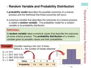
Random Variables • A random variable is a variable whose value is a numerical outcome of a random phenomenon. • For example: Flip three coins and let X represent the number of heads. X is a random variable. • We usually use capital letters to denotes random variables.
Random Variables • A random variable is a variable whose value is a numerical outcome of a random phenomenon. • For example: Flip three coins and let X represent the number of heads. X is a random variable. • The sample space S lists the possible values of the random variable X
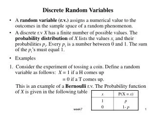
Discrete Random Variable • A discrete random variable X has a countable number of possible values. • For example: Flip three coins and let X represent the number of heads. X is a discrete random variable. • We can use a table to show the probability distribution of a discrete random variable.
Probability Distribution Table: Number of Heads Flipping 4 Coins
Discrete Probability Distributions • Can also be shown using a histogram AP Statistics, Section 7.1, Part 1
What is… • The probability of at most 2 heads? • P(X≤3) = P(X=0) + P(X=1) + P(X=2) + P(X=3) • = 0.0625 + 0.25 + 0.375 + 0.25 • = 0.9375 • OR you could use the complement rule • P(X≤3) =1- P(4) AP Statistics, Section 7.1, Part 1
Example: Maturation of College Students • In an article in the journal Developmental Psychology (March 1986), a probability distribution for the age X (in years) when male college students begin to shave regularly is shown: • Is this a valid probability distribution? How do you know? • What is the random variable of interest? • X= the age in years when male college student begin shaving • Is the random variable discrete? • Yes AP Statistics, Section 7.1, Part 1
Example: Maturation of College Students • In an article in the journal Developmental Psychology (March 1986), a probability distribution for the age X (in years) when male college students begin to shave regularly is shown: • What is the most common age at which a randomly selected male college student began shaving? • What is the probability that a randomly selected male college student began shaving at age 16? • P(X=16) = 0.267 • What is the probability that a randomly selected male college student was at least 13 before he started shaving? • P(X≥13) = 1 – P(X=11) = 1 – 0.013 = 0.987 AP Statistics, Section 7.1, Part 1
Continuous Random Variable • A continuous random variableX takes all values in an interval of numbers.
Distribution of Continuous Random Variable • The probability distribution of X is described by a density curve. • The probability of any event is the area under the density curve and above the values of X that make up that event. • The probability that X = a particular value is 0
Distribution of a Continuous Random Variable • There are two ways to find the given probability. • (1) Find the area less than 0.5 and greater than 0.8, then add them • (2) Find the area between 0.5 and 0.8 and subtract that answer from 1.
Density Curves What density curve have you already learned about? The Normal distribution!
Normal distributions as probability distributions • Suppose X has N(μ,σ) then we can use our tools to calculate probabilities. • One tool we will need is our formula for standardizing variables: Z = X – μ σ
Do you remember?--p.141 The annual rate of return on stock indexes is approximately Normal. Since 1945, the Standard & Poors index has had a mean yearly return of 12%, with a standard deviation of 16.5%. In what proportion of years does the index gain 25% or more? AP Statistics, Section 7.1, Part 1
Do you remember? --p.143 The annual rate of return on stock indexes is approximately Normal. Since 1945, the Standard & Poors index has had a mean yearly return of 12%, with a standard deviation of 16.5%. In what proportion of years does the index gain between 15% and 22%? AP Statistics, Section 7.1, Part 1
Cheating in School • A sample survey puts this question to an SRS of 400 undergraduates: “You witness two students cheating on a quiz. Do you do to the professor?” Suppose if we could ask all undergraduates, 12% would answer “Yes” • We will learn in Chapter 9 that the proportion p=0.12 is a population parameterand that the proportion ô of the sample who answer “yes” is a statistic used to estimate p. • We will see in Chapter 9 that ô is a random variable that has approximately the N(0.12, 0.016) distribution. • The mean 0.12 of the distribution is the same as the population parameter. The standard deviation is controlled mainly by the sample size.
Continuous Random Variable • P-hat (proportion of the sample who answered drugs) is a random variable that has approximately the N(0.12, 0.016) distribution. • What is the probability that the poll result differs from the truth about the population by more than two percentage points? (p=0.12) • P(p-hat<0.10 or p-hat>0.14)
= 1 – (0.10 – 0.12 ≤ p-hat-0.12 ≤ 0.14-0.12) • 0.016 0.016 0.016 • = 1 – (-1.25 ≤ Z ≤ 1.25) • = 1 – (0.8944 – 0.1056) • = 1 – (0.7888) • = 0.2112 • P(p-hat<0.10 or p-hat>0.14) • Let’s start with the complement rule • P(p-hat<0.10 or p-hat>0.14) = 1 – (0.10≤p-hat≤0.14)
Check Point Discrete (a) vs. Continuous (b) You flip a coin and count the number of tails you get in 30 trials. You have each student in Stats run a mile and calculate the time in seconds. You count the number of cookies an SRS of 30 students can eat in one minute. AP Statistics, Section 7.1, Part 1
Check Point P-hat (proportion of the sample who answered drugs) is a random variable that has approximately the N(0.12, 0.016) distribution. What is the probability that the poll result is greater than 13%? What is the probability that the poll result is less than 10%? AP Statistics, Section 7.1, Part 1
Random Variables: MEAN • The Michigan Daily Game you pick a 3 digit number and win $500 if your number matches the number drawn. • There are 1000 three-digit numbers, so you have a probability of 1/1000 of winning • Taking X to be the amount of money your ticket pays you, the probability distribution is: Payoff X: $0 $500 Probability: 0.999 0.001 • We want to know your average payoff if you were to buy many tickets. • Why can’t we just find the average of the two outcomes (0+500/2 = $250?
Random Variables: Mean • So…what is the average winnings? (Expected long-run payoff) Payoff X: $0 $500 Probability: 0.999 0.001
Random Variables: Mean The mean of a probability distribution
Random Variables: Example • The Michigan Daily Game you pick a 3 digit number and win $500 if your number matches the number drawn. • You have to pay $1 to play • What is the average PROFIT? • Mean = Expected Value Payoff X: -$1 $499 Probability: 0.999 0.001
Random Variables: Variance (the average of the squared deviation from the mean) The standard deviationσ of X is the square root of the variance
Random Variables: Example • The Michigan Daily Game you pick a 3 digit number and win $500 if your number matches the number drawn. • The probability of winning is .001 • What is the variance and standard deviation of X?
Technology • When you work with a larger data set, it may be a good idea to use your calculator to calculate the standard deviation and mean. • Enter the X values into List1 and the probabilities into List 2. Then 1-Var Stats L1, L2 will give you μx (as x-bar) and σx (to find the variance, you will have to square σx) • EX: find μx and σ2x for the data in example 7.7 (p.485)
Exercise… • Pretend to “simulate” tossing a fair coin 10 times and write down the results. AP Statistics, Section 7.2, Part 1
Law of Large Numbers • Draw independent observations at random from any population with finite mean μ. • Decide how accurately you would like to estimate μ. • As the number of observations drawn increases, the mean x-bar of the observed values eventually approaches the mean μ of the population as closely as you specified and then stays that close.
Example • The distribution of the heights of all young women is close to the normal distribution with mean 64.5 inches and standard deviation 2.5 inches. • What happens if you make larger and larger samples…
Law of Small Numbers • Most people incorrectly believe in the law of small numbers. • “Runs” of numbers, etc.
Assignment: Exercises: 7.3, 7.7, 7.9, 7.12-7.15, 7.24, 7.27, 7.32-7.34