Download

1 / 45
460 likes | 2.78k Views
Learn the purpose, benefits, and step-by-step process of Analysis of Variance (ANOVA) for statistical data analysis. Understand why ANOVA is preferable over repeated t-tests and how to calculate test statistics effectively.

E N D
ANALYSIS OF VARIANCE (ANOVA) Heibatollah Baghi, and Mastee Badii
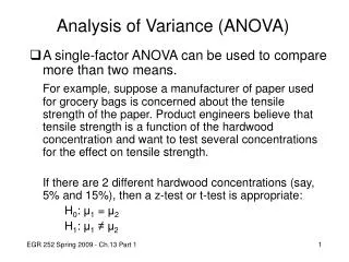
Purpose of ANOVA • Use one-way Analysis of Variance to test when the mean of a variable (Dependent variable) differs among three or more groups • For example, compare whether systolic blood pressure differs between a control group and two treatment groups
Continued Purpose of ANOVA • One-way ANOVA compares three or more groups defined by a single factor. • For example, you might compare control, with drug treatment with drug treatment plus antagonist. Or might compare control with five different treatments. • Some experiments involve more than one factor. These data need to be analyzed by two-way ANOVA or Factorial ANOVA. • For example, you might compare the effects of three different drugs administered at two times. There are two factors in that experiment: Drug treatment and time.
Why not do repeated t-tests? • Rather than using one-way ANOVA, you might be tempted to use a series of t tests, comparing two groups each time. Don’t do it. • Repeated t-test increase the chances of type I error or multiple comparison problem • If you are making comparison between 5 groups, you will need 10 comparison of means • When the null hypothesis is true the probability that at least 1 of the 10 observed significance levels is less than 0.05 is about 0.29
Continued Why not do repeated t-tests? • With 10 means (45 comparisons), the probability of finding at least one significant difference is about 0.63 • In other words, when level of significance is .05, there is a 1 in 20 chance that one t-test will yield a significant result even when the null hypothesis is true. • The more t-test the more that probability will increase
What Does ANOVA Do? • ANOVA involves the partitioning of variance of the dependent variable into different components: • A. Between Group Variability • B. Within Group Variability • More Specifically, The Analysis of Variance is a method for partitioning the Total Sum of Squares into two Additive and independent parts.
Definition of Total Sum of Squares or Variance Grand average Summed acrossall n times p observations
Grand average Average of group j .j Definition of Between Sum of Squares Sum of squared differences of group means from the grand mean is SSB
Group mean Observations Definition of Within Sum of Squares Sum of squareddifference of observations from group means
Total sum of squares Within groups sum of squares Between groups sum of squares Partitioning of Variance into Different Components
Test Statistic in ANOVA Test statistic for ANOVA is based on between & within groups SS
Continued Test Statistic in ANOVA • F = Between group variability / Within group variability • The source of Within group variability is the individual differences. • The source of Between group variability is effect of independent or grouping variables. • Within group variability is sampling error across the cases • Between group variability is effect of independent groups or variables
Steps in Test of Hypothesis • Determine the appropriate test • Establish the level of significance:α • Determine whether to use a one tail or two tail test • Calculate the test statistic • Determine the degree of freedom • Compare computed test statistic against a tabled/critical value Same as Before
Continued 1. Determine the Appropriate Test • Independent random samples have been taken from each population • Dependent variable population are normally distributed (ANOVA is robust with regards to this assumption) • Population variances are equal (ANOVA is robust with regards to this assumption) • Subjects in each group have been independently sampled
2. Establish Level of Significance • α is a predetermined value • The convention • α = .05 • α = .01 • α = .001
3. Use a Two Tailed Test • Ho: 1 = 2 = 3 = 4 Where • 1 = population mean for group 1 • 2 = population mean for group 2 • 3 = population mean for group 3 • 4 = population mean for group 4 • H1 = not Ho
Continued 3. Use a Two Tailed Test • Ha = not Ho • The alternative hypothesis does not specify whether • 1 2 or • 2 3 or • 1 3
4. Calculating Test Statistics • F = (SSb / dfB) / (SSw / dfw) Degrees of freedom between Degrees of freedom within Sum of square between Sum of square within
Continued 4. Calculating Test Statistics • By dividing the sum of the squared deviations by degrees of freedom, we are essentially computing an “average” (or mean) amount of variation • The specific name for the numerator of the F statistic is the mean square between (the average amount of between-group variation • The specific name for the denominator of the F statistic is the mean square within (the average amount of within- group variation)
5. Determine Degrees of Freedom • Degrees of freedom between • dfB = k – 1 • K = number of groups • Degrees of freedom within • dfw = N – k • N = total number of subjects in the study
6. Compare the Computed Test Statistic Against a Tabled Value • α = .05 • If Fc > Fα Reject H0 • If Fc > Fα Can not Reject H0
Example • Suppose we had patients with myocardial infarction in the following groups: • Group 1: A music therapy group • Group 2: A relaxation therapy group • Group 3: A control group • 15 patients are randomly assigned to the 3 groups and then their stress levels are measured to determine if the interventions were effective in minimizing stress.
Continued Example • Dependent Variable • The stress scores. The ranges are from zero (no stress) to 10 (extreme stress) • Independent Variable or Factor • Treatment Conditions(3 levels)
Group 1 average Group 2 average Group 3 average Number of cases Grand average SS Between
Components of Variance SSTotal = SSBetween + SSWithin 116 = 70 + 46
Degrees of Freedom • Df between = 3 -1 • Df within = 15 - 3 dfB = k – 1 dfw = N – k
Test Statistic MSBetween= 70 / 2 = 35 MSWithin= 46 / 12 = 3.83 Fc = MSBetween / MSWithin Fc = 35 / 3.83 = 9.13
Lookup Critical Value • Fα = 3.88
Conclusions • Fc = 9.13 > Fα= 3.88 • Fc > Fα Therefore Reject H0
Multiple Comparison Groups F test does not tell which pair are not equal Additional analysis is necessary to answer which pair are not equal
Fisher’s LSD Test • These are the null and alternative hypothesis being tested • Ho1 : µ1 = µ2 Ha1 : µ1 µ2 • Ho2 : µ1 = µ3 Ha2 : µ1 µ3 • Ho3 : µ2 = µ3 Ha3 : µ2 µ3
Fisher’s LSD Test • Known as the protected t-test • The least difference between means needed for significance • Df = N – K • Use the following formula:
Calculation of LSD • All pairs for means differing by at least 2.70 points on the stress scale would be significantly different from on another.
Application to Three Samples Mean 1 – Mean 2 = 1 Mean 3 – Mean 1 = 4 Mean 3 – Mean 2 = 5 Alternative Hypotheses: Ho1 :µ1 = µ2 Not Rejected Ho2 :µ1 = µ3 Rejected Ho3 :µ2 = µ3 Rejected
N Mean Std. Deviation Std. Error 95% Confidence Interval for Mean Minimum Maximum Lower Bound Upper Bound Music Therapy 5 3.00 2.236 1.000 .22 5.78 0 6 Relaxation Therapy 5 2.00 1.581 .707 .04 3.96 0 4 Control Group 5 7.00 2.000 .894 4.52 9.48 5 10 Total 15 4.00 2.878 .743 2.41 5.59 0 10 SPSS Output for ANOVA Descriptives Stress Levels
Levene Statistic df1 df2 Sig level or p-value .242 2 12 .788 Sum of Squares df Mean Square F Sig.level or p-value Between Groups 70.000 2 35.000 9.130 .004 Within Groups 46.000 12 3.833 Total 116.000 14 SPSS Output for ANOVA Test of Homogeneity of Variances Stress Levels. P > .05, therefore, th assumption of Homogeneity of Variance is met. Stress Levels ANOVA P<.05, therefore, we reject the Null Hypothesis and continue with Multiple Comparison Table
(I) Groups (J) Groups Mean Difference (I-J) Std. Error Sig. Level 95% Confidence Interval Music Therapy Relaxation Therapy 1.000 1.238 .435 -1.70 3.70 Control Group -4.000(*) 1.238 .007 -6.70 -1.30 Relaxation Therapy Music Therapy -1.000 1.238 .435 -3.70 1.70 Control Group -5.000(*) 1.238 .002 -7.70 -2.30 Control Group Music Therapy 4.000(*) 1.238 .007 1.30 6.70 Relaxation Therapy 5.000(*) 1.238 .002 2.30 7.70 SPSS Output for ANOVA Multiple Comparisons Dependent Variable: Stress Levels LSD * The mean difference is significant at the .05 level.
Take home lesson How to compare means of three or more samples