Stability and accuracy of the EM methodology

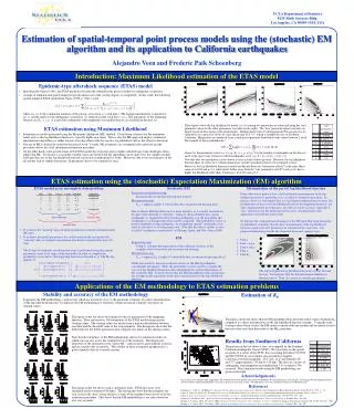
1. UCLA Department of Statistics8125 Math Sciences Bldg. Los Angeles, CA 90095-1554, USA Estimation of spatial-temporal point process models using the (stochastic) EM algorithm and its application to California earthquakes Alejandro Veen and Frederic Paik Schoenberg Introduction: Maximum Likelihood estimation of the ETAS model Epidemic-type aftershock sequence (ETAS) model • Introduced by Ogata (1988), the ETAS model has become the standard point process model for earthquake occurrences • A range of temporal and spatial-temporal specifications exist with varying degrees of complexity. In this work, the following spatial-temporal ETAS model from Ogata (1998, p. 384) is used: where λ(x,y,t) is the conditional intensity of the process at location (x,y) and time t. The background intensity is denoted as μ(x,y) and the index for the earthquake occurrences i is ordered in time, such that ti ≤ ti+1. The parameters of the triggering function are K0, a, c, p, d, q and only earthquakes with magnitudes not smaller than m0 are included in the data set. ETAS estimation using Maximum Likelihood • Estimation is usually performed using the Maximum Likelihood (ML) method. Closed form solutions for the maximum rarely exist as the log-likelihood function is typically highly non-linear. This is why the ML approach employs numerical maximization algorithms (or rather minimization algorithms with the negative log-likelihood (nll) as the objective function). • The use of ML is backed by extensive theoretical work. Usually, ML estimators are (asymptotically) unbiased and the procedure allows for a full-information estimation procedure. • On the other hand, some specifications of the ETAS model have become quite complex which brings some challenges when employing ML. For instance, reasonable starting values are needed and the algorithms can be quite slow for complex models and large data sets as the log-likelihood function can be flat or multimodal (or both). Moreover, due to the non-linearity of the nll and the lack of simple derivatives, all parameters have to be estimated at once. These figures show the log-likelihood of model λ(x,y,t) varying two parameters at a time and using the ‘true’ parameter values for the other parameters (see table on the right). The ‘true’ parameter values (red dot) are largely based on discussions with seismologists. Background events of a homogeneous Poisson process are simulated over a period of about 20 years and an area of 8°×5°, which is roughly the size of Southern California. Magnitudes are simulated from a truncated exponential distribution with values between 2 and 8. The formula of the log-likelihood iswhere θis the parameter vector (i.e. θ = (μ, K0, a, c, p, d, q)), N is the number of earthquakes in the data set, and S is the space-time window in which earthquakes occur (i.e. S = [xl, xr]×[yl, yr]×[tl, tr]). Note that only two parameters can be shown at once in each of these pictures. However, the log-likelihood function takes on values in a 7-dimensional space and all 7 parameters have to be estimated at once. Moreover, the log-likelihood function is relatively flat and there are “interaction effects” in the sense that a value of d=0.08 and q=2.3, while much farther away from the ‘true’ parameters d=0.015 and q=1.8, have a higher log-likelihood value than, for instance, d=0.014 and q=1.9. ETAS estimation using the (stochastic) Expectation Maximization (EM) algorithm ETAS model as an incomplete data problem • If we knew the “missing” data, all model parameters could be estimated easily (M-step) • If we knew the model parameters, we could stochastically reconstruct the “missing” data, or compute expectations (stochastic reconstruction step or E-step) The E-step (or stochastic reconstruction step) is performed using the current parameter vector θs (at step s of the algorithm) in order to compute the probability vector below (the triggering function is denoted as g). The M-step updates θ. Stochastic EM Stochastic reconstruction step Stochastically reconstruct missing data using θs Maximization-step θs+1 = argmaxθ loglik( θ | observable data, reconstructed missing data) The stochastic EM algorithm may be more intuitive, as it actually reconstructs the part of the data that is “missing”. Using θs, the probability that a given earthquake i is triggered by the preceding earthquake j (or the probability that earthquake i is a background event) can be computed. This probability vector is used to randomly assign earthquake i to a triggering “parent” earthquake or in order to classify it as a background event. Note that this idea is similar to what is called “stochastic reconstruction” in Zhuang, Ogata, and Vere-Jones (2004). EM Expectation-step Using θs, compute the expectation of the sufficient statistics of the complete data (observable and reconstructed missing) Maximization-step θs+1 = argmaxθ Eθs [ loglik( θ | observable data, reconstructed missing data) ]While less intuitive, the non-stochastic version of the EM algorithm has considerable advantages. Here, the probability vector is used to compute the expected log-likelihood function, thus eliminating the random fluctuations of the stochastic EM. It can be shown that the EM algorithm provides results that are asymptotically equivalent to the direct maximization of the log-likelihood function. Maximization of the partial log-likelihood function From a theoretical point of view, a full information maximization of the log-likelihood function is preferable as it is an efficient estimation procedure. In practice, however, with limited data sets and limited computational resources, the maximization of the partial log-likelihood based on the triggering function is not only computationally less expensive, but often also more accurate, especially if ‘nice’ expressions for the partial derivatives exist. Asymptotically, both approaches will yield the same results. To illustrate the computational advantages of the EM algorithm using the partial log-likelihood, remember that the direct maximization of the log-likelihood function requires that all 7 parameters be estimated at the same time. Our proposed methodology breaks the estimation down into separate steps: • Find μ • Find c and p • Find d and q • Find a • Find K0 “missing” data observable data complete data The expected partial log-likelihood function is not as flat and has less ‘interactions’ than the full-information likelihood function above. Thus, it is easier to estimate parameters. Applications of the EM methodology to ETAS estimation problems Stability and accuracy of the EM methodology In general, the EM methodology yields results which are extremely close to the parameter estimates of a direct maximization of the log-likelihood function. In addition, the EM methodology is extremely robust and doesn’t depend very much on starting values. The figure on the left shows histograms for the six parameters of the triggering function. They are based on 100 estimations of the ETAS model using random starting values. The starting values are drawn from a uniform distribution between one third and the threefold value of the true parameter. The histograms show that the EM results for the ETAS parameters don’t depend very much on the starting values. Note that the robustness of the EM methodology allows for simulation studies in which one can also assess the standard errors of the estimates. The theoretical properties of the estimators in the “direct ML” context can be quite difficult to derive and are usually only asymptotic. The validity of these asymptotic properties for a given (limited) data set is mostly unclear. The figure on the left shows such a simulation study. ETAS processes were simulated and re-estimated 100 times. The histograms show that the estimates are very close to the ‘true’ values and give a sense of the standard errors involved in this estimation procedure. This shows that the EM methodology is not only robust but also very accurate. Estimation of K0 The figure on the left shows that the EM algorithm (blue) performs better when estimating K0 compared to a direct maximization of the log-likelihood function (orange). Using the same starting values (black circles) the EM results coincide with one another and are much closer to the true value (red) than the results of the ML procedure. Results from Southern California The picture on the left shows a data set compiled by the Southern California Earthquake Center (SCEC). We focus here on the spatial locations of a subset of the SCEC data occurring between 1/01/1984 and 06/17/2004 in a rectangular area around Los Angeles, California, between longitudes -122° and -114° and latitudes 32° and 37° (approximately 733 km by 556 km). The data set consists of earthquakes with magnitude not smaller than 3:0, of which 6,796 occurred. The estimation results using the EM methodology are given on the right. Acknowledgements This material is based upon work supported by the National Science Foundation under Grant No. 0306526. We thank Yan Kagan, Ilya Zaliapin, and Yingnian Wu for helpful comments and the Southern California Earthquake Center for its generosity in sharing its data. All computations have been performed using R (www.R-project.org). References Dempster, A., Laird, N., and Rubin, D., Maximum likelihood from incomplete data via the EM algorithm, Journal of the Royal Statistical Society, Series B, 39/1, , 1977, 1 – 38. Ogata, Y., Statistical Models for Earthquake Occurrences and Residual Analysis for Point Processes, Journal of the American Statistical Association, Vol. 83, 1988, 9 – 27. Ogata, Y., Space-time point-process models for earthquake occurrences, Annals of the Institute of Statistical Mathematics, Vol. 50, 1998, 379 – 402. Sornette, D. and Werner, M.J., Apparent Clustering and Apparent Background Earthquakes Biased by Undetected Seismicity, J. Geophys. Res., Vol. 110. Zhuang, J., Y. Ogata, and D. Vere-Jones (2002), Stochastic declustering of space-time earthquake occurrences, Journal of American Statistical Association, Vol. 97, No. 458, 369 – 380. Zhuang, J., Y. Ogata, and D. Vere-Jones (2004), Analyzing earthquake clustering features by using stochastic reconstruction, J. Geophys. Res., Vol. 109.