Download
1 / 41
430 likes | 786 Views
Geometry Optimization, Molecular Dynamics and Vibrational Spectra. Pablo Ordejón ICMAB-CSIC. Born-Oppenheimer dynamics. Nuclei are much slower than electrons. electronic. decoupling. nuclear. Classical Nuclear Dynamics. Optimization and MD basic cycle.

E N D
Geometry Optimization, Molecular Dynamics and Vibrational Spectra Pablo Ordejón ICMAB-CSIC
Born-Oppenheimer dynamics Nuclei are much slower than electrons electronic decoupling nuclear Classical Nuclear Dynamics
Extracting information from the Potential Energy Surface (PES) • Optimizations and Phonons: • We move on the PES • Local vs global minima • PES is harmonic close to min. • MD • We move over the PES (KE) • Good Sampling is required!!
Theory of geometry optimization Gradients Hessian =1 for quadratic region
Energy only: simplex Energy and first derivatives (forces): steepest descents (poor convergence) conjugate gradients (retains information) approximate Hessian update Energy, first and second derivatives Newton-Raphson Broyden (BFGS) updating of Hessian (reduces inversions) Rational Function Optimisation (for transition states/and soft modes) Methods of Optimisation SIESTA presently uses conjugate gradients and BFGS
Steepest Descents • Start at xo • Calculate gradient g(x) = f(x) • Minimize f(x) along the line defined by the gradient • Start again until tolerance is reached
Steepest Descents Performance depends on • Eigenvalues of Hessian (λmax / λmin) • Starting point
Conjugate Gradients • Same idea, but retaining information about previous steps • Search directions ‘conjugate’ (orthogonal) to previous • Convergence assured for N steps See “Numerical Recipes” by Press et al (Cambridge) for details
Using the Hessian • Energy, first and second derivatives: - Newton-Raphson: An approximation of H at a position (Xk) is calculated. Then finding the inverse of that Hessian (H-1), and solving the equation P = -H-1*F(Xk) gives a good search direction P. Later, a line search procedure has to determine just how much to go in that direction (producing the scalar alpha). The new position is given by: Xk+1 = Xk + alpha*P • Broyden (BFGS): updating of an approximateHessian Basic idea, update the Hessian along the minimization to fit: ... using only the forces!!
Set runtype to conjugate gradients or Broyden: MD.TypeOfRun CG, Broyden Set maximum number of iterative steps: MD.NumCGsteps 100 Optionally set force tolerance: MD.MaxForceTol 0.04 eV/Ang Optionally set maximum displacement: MD.MaxCGDispl 0.2 Bohr Optimization Variables in SIESTA(1)
By default: optimisations are done for a fixed cell To allow unit cell to vary: MD.VariableCell true Optionally set stress tolerance: MD.MaxStressTol 1.0 Gpa Optionally set cell preconditioning: MD.PreconditionVariableCell 5.0 Ang Set an applied pressure: MD.TargetPressure 5.0 GPa Optimization Variables in SIESTA(2)
Make sure that your MeshCutoff is large enough: - Mesh leads to space rippling - If oscillations are large convergence is slow - May get trapped in wrong local minimum Advice on Optimizations in SIESTA(I)
Advice on Optimizations in SIESTA(II) • Ill conditioned systems (soft modes) can slow down optimizations, very sensitive to mesh cuttoff. - Use constraints when relevant. Fixed to Si Bulk
Advice on Optimizations in SIESTA(III) • Decouple Degrees of freedom (relax separately different parts of the system). • Look at the evolution of relevant physics quantities (band structure, Ef). Fix the Zeolite, Its relaxation is no Longer relevant. Ftube<0.04 eV/A Fzeol>0.1 eV/A No constraints
Optimise internal degrees of freedom first Optimise unit cell after internals Exception is simple materials (e.g. MgO) Large initial pressure can cause slow convergence Small amounts of symmetry breaking can occur Check that geometry is sufficiently converged (as opposed to force - differs according to Hessian) SCF must be more converged than optimisation Molecular systems are hardest to optimise More Advice on Optimisation…..
The following can currently be constrained: - atom positions - cell strains - Z-matrix (internal coordinates) User can create their own subroutine (constr) To fix atoms: To fix stresses: Using Constraints Stress notation: 1=xx, 2=yy, 3=zz, 4=yz, 5=xz, 6=xy
Molecular Dynamics • Follows the time evolution of a system • Solve Newton’s equations of motion: • Treats electrons quantum mechanically • Treats nuclei classically • Hydrogen may raise issues: tunnelling, zero point E... • Allows study of dynamic processes • Annealing of complex materials • Influence of temperature and pressure • Time averages vs Statistical averages
Ergodicity • In MD we want to replace a full sampling on the appropriate statistical ensemble by a SINGLE very long trajectory. • This is OK only if system is ergodic. • Ergodic Hypothesis: a phase point for any isolated system passes in succession through every point compatible with the energy of the system before finally returning to its original position in phase space. This journey takes a Poincare cycle. • In other words, Ergodic hypothesis: each state consistent with our knowledge is equally “likely”. • Implies the average value does not depend on initial conditions. • <A>time= <A>ensemble , so <Atime> = (1/NMD) = ∑t=1,N At is good estimator. • Are systems in nature really ergodic? Not always! • Non-ergodic examples are glasses, folding proteins (in practice) and harmonic crystals (in principle).
The system relaxes on a “reasonable” time scale towards a unique equilibrium state (microcanonical state) Trajectories wander irregularly through the energy surface eventually sampling all of accesible phase space. Trajectories initially close together separate rapidily (Sensitivity to initial conditions). Ergodic behavior makes possible the use of statistical methods on MD of small system. Small round-off errors and other mathematical approximations should not matter. Different aspects of ergodicity
Particle in a smooth/rough circle From J.M. Haile: MD Simulations
Molecular Dynamics(I) In Molecular Dynamics simulations, one computes the evolution of the positions and velocities with time, solving Newton’s equations. • Algorithm to integrate Newton’s equations: “Verlet” • Initial conditions in space and time.
Initialize positions and momenta at t=0 (initial conditions in space and time) Solve F = ma to determine r(t), v(t). (integrator) We need to make time discrete, instead of continuous!!! Calculate the properties of interest along the trajectory Estimate errors Use the results of the simulation to answer physical questions!!. Molecular Dynamics(II) h=t t0 t1 t2 tn-1 tn tn+1 tN
Timestep must be small enough to accurately sample highest frequency motion Typical timestep is 1 fs (1 x 10-15 s) Typical simulation length: Depends on the system of study!! (the more complex the PES the longer the simulation time) Is this timescale relevant to your process? Simulation has two parts equilibration – when properties do not depend on time production (record data) Results: diffusion coefficients Structural information (RDF’s,) Free energies / phase transformations (very hard!) Is your result statistically significant? Molecular Dynamics III
The most commonly used algorithm: r(t+h) = r(t) + v(t) h + 1/2 a(t) h2 + b(t) h3 + O(h4) (Taylor series expansion) r(t-h) = r(t) - v(t) h + 1/2 a(t) h2 - b(t) h3 + O(h4) r(t+h) = 2 r(t) - r(t-h) + a(t) h2 + O(h4) Sum v(t) = (r(t+h) - r(t-h))/(2h) + O(h2) Difference (estimated velocity) Trajectories are obtained from the first equation. Velocities are not necessary. Errors in trajectory: O(h4) Preserves time reversal symmetry. Excellent energy conservation. Modifications and alternative schemes exist (leapfrog, velocity Verlet), always within the second order approximation Higher order algorithms: Gear Integrator: Verlet algorithm
NVE (Verlet): Microcanonical. Integrates Newtons equations of motion, for N particles, in a fixed volume V. Natural time evolution of the system: E is a constant of motion Different ensembles: conserved magnitudes Same sampling In the thermodynamic limit • NVT (Nose): Canonical • System in thermal contact with a heat bath. • Extended Lagrangian: • N particles + Thermostat, mass Q. • NPE (Parrinello-Rahman) (isobaric) • Extended Lagrangian • Cell vectors are dynamical variables with an associated mass. • NPT (Nose-Parrinello-Rahman) • 2 Extended Lagrangians • NVT+NPE.
MD in canonical distribution (TVN) Introduce a friction force (t) Nose-Hoover thermostat SYSTEM T Reservoir Dynamics of friction coefficient to get canonical ensemble. Feedback makes K.E.=3/2kT Q= fictitious “heat bath mass”. Large Q is weak coupling
Nose Mass: Match a vibrational frequency of the system, better high energy frequency Hints
MD.TypeOfRun Verlet NVE ensemble dynamics MD.TypeOfRun Nose NVT dynamics with Nose thermostat MD.TypeOfRun ParrinelloRahman NPE dynamics with P-R barostat MD.TypeOfRun NoseParrinelloRahman NPT dynamics with thermostat/barostat MD.TypeOfRun Anneal Anneals to specified p and T Molecular Dynamics in SIESTA(1) VariableCell
Setting the length of the run: MD.InitialTimeStep 1 MD.FinalTimeStep 2000 Setting the timestep: MD.LengthTimeStep 1.0 fs Setting the temperature: MD.InitialTemperature 298 K MD.TargetTemperature 298 K Setting the pressure: MD.TargetPressure 3.0 Gpa Thermostat / barostat parameters: MD.NoseMass / MD.ParrinelloRahmanMass Molecular Dynamics in SIESTA(2) Maxwell-Boltzmann
MD can be used to optimize structures: MD.Quench true - zeros velocity when opposite to force MD annealing: MD.AnnealOption Pressure MD.AnnealOption Temperature MD.AnnealOption TemperatureAndPressure Timescale for achieving target MD.TauRelax 100.0 fs Annealing in SIESTA
SystemLabel.MDE conserved quantity SystemLabel.MD (unformatted; post-process with iomd.F) SystemLabel.ANI (coordinates in xyz format) If Force Constants run: SystemLabel.FC Output Files
Visualisation and Analysis Molekel http://www.cscs.ch/molekel XCRYSDEN http://www.xcrysden.org/ GDIS http://gdis.seul.org/
Calculating Dynamical Matrix: Mass weighted Hessian Matrix Frozen Phonon approximation: Numerical evaluation of the second derivatives. (finite differences). Density Functional Perturbation Theory (Linear Response): Perturbation theory used to obtain analytically the Energy second derivatives within a self consistent procedure. Molecular dynamics: Green-Kubo linear response. Link between time correlation functions and the response of the system to weak perturbations. Vibrational spectra: Phonons Harmonic Approx. Beyond Harmonic Approx.
Frozen Phonon approximation: MD.TypeOfRun FC MD.FCDispl 0.04 Bohr (default) Total number of SCF cycles: 3 X 2 X N = 6N (x,y,z) (+,-) Nat Output file: SystemLabel.FC Building and diagonalization of Dynamical matrix: VibraSuite (Vibrator) (in /Util) Phonons in Siesta (I)
Phonons in Siesta (II) Relax the system: Max F<0.02 eV/Ang Increase MeshCutof, and run FC. 3. If possible, test the effect of MaxFCDispl.
Phonons and MD • MD simulations (NVE) • Fourier transform of Velocity-Velocity autocorrelation function. • Anharmonic effects: (T) • Expensive, but information available for MD simulations.