Download
1 / 50
500 likes | 656 Views
Overview of Gene Clustering and Algorithmic Methodologies. Beth Benas Rizwan Habib Alexander Lowitt Piyush Malve. Contents. What is Gene Clustering?. Two or more genes that code for the same or similar products Two different processes for duplication of original genes via:

E N D
Overview of Gene Clustering and Algorithmic Methodologies Beth Benas RizwanHabib Alexander Lowitt PiyushMalve
What is Gene Clustering? • Two or more genes that code for the same or similar products • Two different processes for duplication of original genes via: 1) Homologous recombination 2) Transposition events
Homologous Recombination • Genetic recombination where nucleotides are exchanged between similar or identical strands of DNA • Breaking and rejoining strands of DNA • Established in meiosis to provide for more genetic variability
Homologous Recombination *http://www.web-books.com/MoBio/Free/Ch8D1.htm
Misalignment During Homologous Recombination http://jeb.biologists.org/cgi/reprint/203/6/1059.pdf
Retrotransposon • Transposons mobile DNA • Sequences of DNA that are capable of moving to alternative positions along the genome of a single cell • “jumping genes” • Retrotransposition type of transposon able to become amplified within a genome • Relatively stable and tend to withstand natural selection • Thus, prevalent across generations
Mutations in Duplicated Gene • Second copy generated is free from selective pressure • Second copy can mutate quicker • Not necessarily lasting changes
What Does All This Mean? • Useful technique to group similar genetic code together • Relational understanding between homologous objects • Trending / patterns of genetic expression • Functional relatedness • Phenotypic relatedness
What is Gene Clustering? • Presume • Genome is a 2D Cartesian space or a graph paper • Genes are now points on this graph paper • Let see how many lines and hyperbolas are there? • Gene clustering is the process of assigning two or more genes to a “gene cluster” that serve to encode for the same or similar products • As populations from a common ancestor tend to possess the same varieties of gene clusters, they are useful for tracing back recent evolutionary history. • An example of a gene cluster is the Human β-globin gene cluster, which contains five functional genes and one non-functional gene for similar proteins. • All Hemoglobin molecules contain any two identical proteins from this gene cluster, depending on their specific role.
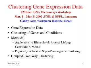
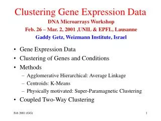
Hierarchical Clustering • Allows organization of the clustering data to be represented in a tree (dendrogram) • Agglomerative (Bottom Up): each observation starts as own cluster. Clusters are merged based on similarities • Divisive (Top Down): all observations start in one cluster, and splits are performed recursively as one moves down the hierarchy. • In general, splits in the tree are determined in a greedy manner.
Hierarchical Clustering Agglomerative Divisive
Hierarchical Clustering • A measure of dissimilarity between sets of observations is required for combination and division of clusters. • This is achieved by use of an appropriate metric (a measure of distance between pairs of observations), and a linkage criteria which specifies the dissimilarity of sets as a function of the pairwise distances of observations in the sets.
Hierarchical Clustering • The choice of an appropriate metric will influence the shape of the clusters, as some elements may be close to one another according to one distance and farther away according to another. • The linkage criteria determines the distance between sets of observations as a function of the pairwise distances between observations.
Advantage • Hierarchical clustering has the distinct advantage that any valid measure of distance can be used. In fact, the observations themselves are not required: all that is used is a matrix of distances
K- Means Clustering • k-means clustering is a method of cluster analysis which aims to partition n observations into k clusters in which each observation belongs to the cluster with the nearest mean. • It is similar to the expectation-maximization algorithm for mixtures of Gaussians in that they both attempt to find the centers of natural clusters in the data.
K- Means Clustering • Regarding computational complexity, the k-means clustering problem is: • NP-hard in general Euclidean space d even for 2 clusters. • NP-hard for a general number of clusters k even in the plane. • If k and d are fixed, the problem can be exactly solved in time O(ndk+1 log n), where n is the number of entities to be clustered. • Thus, a variety of heuristic algorithms are generally used.
K- Means Clustering • Heuristic algorithm no guarantee that it will converge to the global optimum • Algorithm is usually very fast it is common to run it multiple times with different starting conditions. • It has been shown that there exist certain point sets on which k-means takes super polynomial time: 2Ω(√n) to converge.
K- Means Clustering • Two key features of k-means efficiency • The number of clusters k is an input parameter: an inappropriate choice of k may yield poor results. • Euclidean distance is used as a metric and variance is used as a measure of cluster scatter. • Often regarded as its biggest drawbacks.
Applications of K-Means • Image segmentation • The k-means clustering algorithm is commonly used in computer vision as a form of image segmentation. • The results of the segmentation are used to aid border detection and object recognition. • Standard Euclidean distance is usually insufficient in forming the clusters. • Instead, a weighted distance measure utilizing pixel coordinates, RGB pixel color and/or intensity, and image texture is commonly used.
SOM • Self organizing map (SOM) is a learning method which produces low dimension data (e.g. 2D) from high dimension data (nD) • E.g. an apple is different from a banana in more then two ways but they can be differentiated based on their size and color only. • If we present apples and bananas with points and similarity with lines then • Two points connected by a shorter line are of same kind • Two points connected by a longer line are of different kind • Shorter line = line with length less then threshold t • Longer line = line with length greater then threshold t • We just created a map to differentiate an apple from banana based on two traits only. • We have successfully “trained” the SOM, now anyone can use to “map” apples from banana and vice versa • DEMO for SOM Training • DEMO for SOM Mapping
Application of SOM • Genome Clustering • Goal: trying to understand the phylogenetic relationship between different genomes. • Compute: bootstrap support of individual genomes for different phylogentic tree topologies, then cluster based on the topology support. • Clustering Proteins based on the architecture of their activation loops • Align the proteins under investigation • Extract the functional centers • Turn 3D representation into 1D feature vectors • Cluster based on the feature vectors
PCA • Principal component analysis (PCA) is a mathematical procedure that transforms a number of possibly correlated variables into a smaller number of uncorrelated variables called principal components • Also know as Independent component analysis or dimension reduction technique • SOM and PCA are related (SOM is non-linear PCA) • PCA decomposes complex data relationship into simple components and then represent all data in terms of these simple components • SOM is efficient then PCA but PCA is more versatile.
PCA Example • Suppose three entities X1, X2 and X3 acts together to define a process. i.e. their graph will have three dimensions
Apply PCA • It is hard to guess the relationships • X1 vs. X2 • X2 vs. X3 • X3 vs. X1 • PCA can transform this 3D graph into four 2D graph to reveal individual relationship among each of three Xi.
Cluster 3.0 • Implements most commonly used clustering methods for gene expression data analysis • provides a computational and graphical environment for analyzing data from DNA microarray experiments, or other genomic datasets • Data_set.txt => Cluster 3.0 => cluster_output.txt • Cluster_output.txt => TreeView => Visualization • Cluster 3.0, TreeView are both open source and Sample data is also provided to play around with it.
Loading File • Rows are genes • Columns are samples (BLUE) • YOFR (yeast open reading frame) is used by TreeView to specify how rows are linked to external websites • Table is represented as a tab delimited file for Cluster to use it
Filter Data • Filtering tab allows you to remove genes that do not have certain desired properties from your dataset • % Present >= X. This removes all genes that have missing values in greater than (100-X) percent of the columns. • SD (Gene Vector) >= X. This removes all genes that have standard deviations of observed values less than X. • At least X Observations with abs(Val) >= Y. This removes all genes that do not have at least X observations with absolute values greater than Y. • MaxVal-MinVal >= X. This removes all genes whose maximum minus minimum values are less than X.
Adjusting Data • Cluster allow to perform a number of operations that alter the underlying data in the imported file • Log Transform Data: replace all data values x by log2 (x). Why? • Center genes [mean or median]: Subtract the row-wise mean or median from the values in each row of data, so that the mean or median value of each row is 0. • Center arrays [mean or median]: Subtract the column-wise mean or median from the values in each column of data, so that the mean or median value of each column is 0. • Normalize genes: Multiply all values in each row of data by a scale factor S so that the sum of the squares of the values in each row is 1.0 (a separate S is computed for each row). • Normalize arrays: Multiply all values in each column of data by a scale factor S so that the sum of the squares of the values in each column is 1.0 (a separate S is computed for each column). • These operations are not associative, so the order in which these operations is applied is very important • Log transforming centered genes are not the same as centering log transformed genes.
Log Transformation • Experiment: analyzing gene expression data from DNA microarray as florescent ratios • We are looking gene expression over time • Results are relative expression level to time 0 • Time 0: base time • Time 1: gene is unchanged • Time 2: gene is up-regulated 2 folds • Time 3: gene is down-regulated 2 folds • “Is 2-fold up the same magnitude of change as 2-fold down but just in the opposite direction?” • If yes, then log transform the sample data • If no, then use the data as it is
Mean/Median Centering • Experiment: analyzing a large number of tumor samples all compared to a common reference sample made from a collection of cell-lines. • For each gene, you have a series of ratio values that are relative to the expression level of that gene in the reference sample. • Since the reference sample really has nothing to do with your experiment, you want your. • “Is reference sample a part of the experimental samples or vice versa, i.e. analysis is independent of the amount of a gene present in the reference sample” • If yes, then use centering • If no, then work with raw data • Median centering is preferred over mean centering
Distance/Similarity Measure • “Is graph on the left the same as graph on the right?” • Pearson correlation factor says they are similar, i.e. x = 2x = 2x+y. Use Spearman rank correlation or Kendall's τ of Cluster 3.0. • Euclidean distance says they are not similar, i.e. x != 2x. • Pearson measures only the similarity while Euclidean measures the magnitude of similarity.
Article • “Systematic Variation in Gene Expression Patterns in Human Cancer Cell Lines” • 2000: Nature America, Inc.; Princeton University • http://genetics.nature.com • Primary authors • Ross Douglas, ScherfUwe, Michael Eisen
Background • Cell lines from human tumors used for many years as experimental models to show neoplasia or neoplastic disease • 60 cancer cell lines National Cancer Institute’s Developmental Therapeutics Program (DPT) • DNA microarrays to show variation in the prevalence of transcripts • Comparing RNA from: • Two breast cancer biopsy samples • Sample of normal breast tissue • NCI60 cell lines derived from breast cancers (excluding MDA-MB-435 and MDA-N) • Leukaemias • Pattern shared between the cancer specimens and individual cell lines derived from breast cancers and leukaemias
Background • cDNA microarrays were used to explore variation in 8,000 different genes along 60 cell lines • National Cancer Institute • Screen for anti-cancer drugs • Purpose: • Show phenotypic variation cell reproduction rate, drug metabolism • Location of tumors • To verify gene expression comparison patterns in cell lines to that of normal breast tissue or tumor samples within breast tissue • Clustering to look at outliers that would validate or dismiss previous classification efforts
Clustering in Action • Process: Develop rows of genes and columns of microarray hybridization • Normalized fluorescence ratios from the database • Subtraction of local background • Established specific criteria to group a subset of the 9,703 cDNA elements from the arrays • Centered data by subtracting arithmetic mean of all ratios measured • log2 (ratio) > 2.8 • Centering provides for all future analysis to be independent of amount of mRNA in reference pool
Clustering in Action • Display representing microarray hybridization and genes • Normalized the data and switched quantitative data to that of a color gradient • Each color represents the mean adjusted expression level of the gene and cell line
Clustering in Action • Hierarchical clustering algorithm • Pearson correlation coefficient comparing similarities and ignoring differences in variation along cell line genes • Similar expression characterized by short branches and longer branches denote dissimilarities
Clustering in Action • Dendrogram: gene expression patterns within cell line of original tissue • Cell lines derived from leukaemia, melanoma, central nervous system, colon, renal and ovarian tissue.
Conclusions • cDNA’s provided 8,000 genes only 3,700 represented previously classified human proteins • 1,900 had homologues in other organisms and 2,400 were identified via ESTs • Estimated that 80% of the genes were correctly identified • Able to analyze intact tumors within their specific microenvironment • Dendrograms provide possibility improved taxonomy of cancer • Helpful to explain heterogeneity of breast cancer • Possibility of individual treatment regimens (personalized medicine)