Qualitative and Quantitative traits

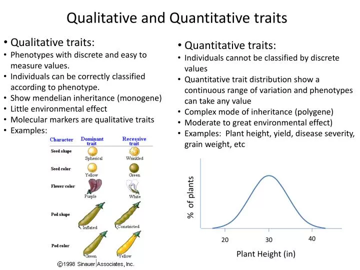
1. Qualitative and Quantitative traits • Qualitative traits: • Phenotypes with discrete and easy to measure values. • Individuals can be correctly classified according to phenotype. • Show mendelian inheritance (monogene) • Little environmental effect • Molecular markers are qualitative traits • Examples: • Quantitative traits: • Individuals cannot be classified by discrete values • Quantitative trait distribution show a continuous range of variation and phenotypes can take any value • Complex mode of inheritance (polygene) • Moderate to great environmental effect) • Examples: Plant height, yield, disease severity, grain weight, etc % of plants 40 20 30 Plant Height (in)

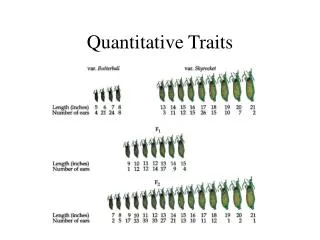
2. Inheritance of Quantitative traits The study of quantitative trait inheritance followed the same steps as for Mendelian traits. At the beginning they were thought to not follow Mendel’s laws. But it is not true • PARENT 1: • pure line, completely homozygote • 40 inches • PARENT 2: • pure line, completely homozygote • 20 inches F1 F1: range of height distribution but no type of segregation F2: wider range of height distribution but no type of segregation F2

3. Inheritance of Quantitative traits In 1903 the Danish botanist Wilhelm Johannsen measured the weight of seeds in the Princess variety of bean. This variety is a pure line since beans are self-fertilizing . From a seed lot he measured and classified the beans by weight and obtained the range of distribution for that variety. Then he selected 19 beans of different weights and self-pollinated them several generations Doing this he got 19 pure lines (completely homozygous) in case they were not at the beginning of the experiment He found that: The weight of the 5,494 beans he obtained followed a normal distribution All lines within each of the 19 groups were genetically identical but showed also a range of variation in weights. The average and distribution of weight in each pure line were similar to those of the original population

4. Inheritance of Quantitative traits The Experiment of Johannsen • Conclusions: • There is a genetic control that keeps the same average weight and distribution • However not all genetically identical seeds have the same weight. • The phenotype of each individual must be determined by the genotype and the environmental conditions • Without genetic variability, genetic improvement is not possible

5. Inheritance of Quantitative traits Johannsen showed that quantitative traits are determined by genes. However he did not find any type of mendelian segregation. This was studied in 1909 by Swedish Herman Nilsson-Ehle who studied kernel color in wheat He had several pure lines of red and white colored kernels. When crossing red x white he got always red F1, but different proportions of red and white kernels depending on the cross: a) 3 red : 1 white b) 15 red : 1 White c) 63 red : 1 white He deduced that the color was controlled by three loci. Only individuals with recessive homozygous alleles at the three loci showed the white phenotype. When a single dominant allele (A, B or C) is present at any of the three loci the red phenotype shows up.

6. Inheritance of Quantitative traits a) 3 red : 1 white b) 15 red : 1 White c) 63 red : 1 white For case a), allelic variation between the two parents was present only at one locus P1 (red) P2 (white) AAbbcc X aabbcc F1(red) Aabbcc ¼ AAbbcc : ½ Aabbcc : ¼ aabbcc F2 (only one locus segregating) (red) (red) (white) Segregation 3 red : 1 white

7. Inheritance of Quantitative traits a) 3 red : 1 white b) 15 red : 1 White c) 63 red : 1 white P1 (red) P2 (white) AABBcc X aabbcc F1(red) AaBbcc 1/16 AABBcc (red) 2/16 AABbcc (red) 1/16 AAbbcc (red) 2/16 AaBBcc (red) 4/16 AaBbcc (red) 2/16 Aabbcc (red) 1/16 aaBBcc (red) 2/16 aaBbcc (red) 1/16 aabbcc (white) F2 (two loci segregating) Segregation 15 red : 1 white

8. Inheritance of Quantitative traits a) 3 red : 1 white b) 15 red : 1 White c) 63 red : 1 white P1 (red) P2 (white) AABBCC X aabbcc F2 (three loci segregating) F1(red) AaBbCc Segregation 63 red : 1 white 1/64 AABBCC (red) 2/64 AABbCC (red) 1/64 AabbCC (red) 2/64AaBBCC (red) 4/64 AaBbCC (red) 2/64 AabbCC (red) 1/64 aaBBCC (red) 2/64 aaBbCC (red) 1/64 aabbCC (red) 2/64 AABBCc (red) 4/64 AABbCc (red) 2/64 AabbCc (red) 4/64 AaBBCc (red) 8/64 AaBbCc (red) 4/64 AabbCc (red) 2/64 aaBBCc (red) 4/64 aaBbCc (red) 2/64 aabbCc (red) 1/64 AABBcc (red) 2/64 AABbcc (red) 1/64 Aabbcc (red) 2/64 AaBBcc (red) 4/64 AaBbcc (red) 2/64 Aabbcc (red) 1/64 aaBBcc (red) 2/64 aaBbcc (red) 1/64 aabbcc (white)

9. Inheritance of Quantitative traits However, Nilsson-Ehle not only classified the seeds by color. He also classified them by color intensity and saw that color intensity also had a defined segregation pattern P1 (purple, very dark red) P2 (white) P1 (purple, X very dark red) P2 (white) AABB X aabb He proposed that for this cross, color intensity was determined by two loci with two alleles each: one that produced red pigment (A and B) and other with no pigment (a and b). He determined that the effects of the alleles were additive and contributed equally to the phenotype, which depended on the number of alleles for pigment present F1(red) AaBb F1(red) 1/16 AABB (Purple) 2/16 AABb (dark-red) 1/16 AAbb (red) 2/16 AaBB (dark-red) 4/16 AaBb (red) 2/16 Aabb (light-red) 1/16 aaBB (red) 2/16 aaBb (light-red) 1/16 aabb (white) 1/16 : purple 4/16: dark-red 6/16: red 4/16: light-red 1/16: white

10. Inheritance of Quantitative traits P1 (purple, X very dark red) P2 (white) Going one step further, He saw that within each of the groups there was also some variation F1(red) Frequency - white + purple Color intensity 1/16 : purple 4/16: dark-red 6/16: red 4/16: light-red 1/16: white

11. Inheritance of Quantitative traits He deduced that many loci were involved (not only two) in the trait and taking into account Johanssen’s findings: Phenotype=Genotype+Environment Then, the distribution of a quantitative trait would follow a normal distribution 4 Frequency 3 2 1 + purple - white Color intensity Analysis of quantitative traits is therefore complicated: Same genotype: 1 and 2 show different phenotype Same phenotype: 1, 3 and 4 is the result of three different genotypes

12. Inheritance of Quantitative traits The inheritance of quantitative traits also explains the phenomenon of transgressive segregation: In the progeny of a cross we can get phenotypes out of the range of the parents P2 P1 0 10 Frequency Let’s assume 5 loci with additive effects control the trait P1 P2 aabbccddEE X AABBCCDDee Cold tolerance AaBbCcDdEe F1 F2 All possible combinations of alleles at 5 loci. Between them: AABBCCDDEE (all favorable alleles) aabbccddee (all unfavorable alleles)

13. Inheritance of Quantitative traits Quantitative traits are usually controlled by several genes with small additive effects and influenced by the environment Heritability h2measures the proportion of phenotypic variation (variance) that is due to genetic causes P = G + E; VP = VG + VE A heritability of 40% for cold tolerance means that within that population, genetic differences among individuals are responsible of 40% of the variation. Therefore, 60% is due to environmental causes. However, that does not mean that the cold tolerance of a certain individual is due 40% to genetic causes and 60% to environmental causes. h2 is a property of the population and not of individuals

14. Inheritance of Quantitative traits Heritability h2measures the proportion of phenotypic variation (variance) that is due to genetic causes P = G + E; VP = VG + VE h2 ranges between 0 and 1 If h2is 0 means : a) The trait is not genetically controlled. All the variation we see is due to environmental factors, or b) The trait is genetically controlled but all individuals have the same genotype h2 is very useful because it allows us to predict the response to artificial selection

15. Inheritance of Quantitative traits Heritability h2measures the proportion of phenotypic variation (variance) that is due to genetic causes P = G + E; VP = VG + VE h2 is very useful because it allows us to predict the response to artificial selection In plant breeding, the starting point is a segregating population (with genetic variability). The best individuals are selected to be the progenitors of the next generation μ0 Selection differential (S) = μS – μ0 Response to selection (R) = μR – μ0 Realized heritability: Is the ratio of the single-generation progress of selection to the selection differential of the parents. The higher h2, the higher the progress of selection in each generation Frequency μS Grain yield (lb/A) 0 6000 μ0 μR Frequency Grain yield (lb/A) 0 6000

16. Analysis of Quantitative traits The analysis of quantitative traits is based on the identification of the individual loci (QTL) controlling the trait, their location, effects and interactions A quantitative trait locus/loci (QTL) is the location of individual locus or multiple loci that affects a trait that is measured on a quantitative (linear) scale. These traits are typically affected by more than one gene, and also by the environment. Thus, mapping QTL is not as simple as mapping a single gene that affects a qualitative trait (such as flower color).

17. Analysis of Quantitative traits There are two main approaches for QTL analysis: a) QTL analysis in mapping populations b) Association mapping Both approaches share a set of common elements: a) A population (array of individuals) that show variability for the trait of study b) Phenotypic information: We need to design an experiment to estimate the phenotypic value of each individual c) Genotypic information: A set of molecular markers that have been run in all the individuals of the population d) A statistical method to estimate QTL position, effects and interactions

18. Analysis of Quantitative traits QTL analysis in mapping populations We need to develop a population from a single cross between two individuals that show contrasting phenotypes for the trait of study. For example, if we want to study quantitative resistance to Barley Stripe Rust (Puccinia striiformis f. sp. Hordei) we will develop a population from the cross between a susceptible line and a resistant line. The offspring of that cross will show recombination between the two parents and therefore, some individuals will be resistant and other will be susceptible Different types of mapping populations can be used: Doubled haploids (DH), Recombinant inbred lines (RIL), F2, Back cross (BC), etc. Always all individuals trace back to a single cross

19. Analysis of Quantitative traits QTL analysis in mapping populations The first step is getting genotypic information for all the individuals of the population: molecular markers P2 P1 Back Cross population P1 P2 High Throughput genotyping platform (SNP)

20. Analysis of Quantitative traits QTL analysis in mapping populations If molecular markers are polymorphic, we can construct a linkage map based on recombination frequencies:

21. Analysis of Quantitative traits QTL analysis in mapping populations The basic QTL analysis method consists in walking trough the chromosomes performing statistical test at the positions of the markers in order to test whether there is a marker-trait association or not

22. Analysis of Quantitative traits Disease severity (%) DsT-66 Average Disease severy of plants with allele “A” (Inherited from Resistant parent) = 49.8 Average Disease severity of plants with allele “B” (Inherited from Susceptible parent) = 50.3 49.8 and 50.3 are not statistically different. Therefore, marker DsT-66 is not associated with resitance/susceptibility to the disease

23. Analysis of Quantitative traits Disease severity (%) ABC261 Average Disease severy of plants with allele “A” (Inherited from Resistant parent) = 30.4 Average Disease severity of plants with allele “B” (Inherited from Susceptible parent) = 69.8 30.4 and 69.8 are statistically different. Therefore, marker ABC261 is linked with a resitance/susceptibility QTL. The additive effect of the QTL is: a = (69.8-30.4)/2 = 14.7

24. Analysis of Quantitative traits QTL analysis in mapping populations Significance trheshold Probability Most likely position of the QTL

25. Analysis of Quantitative traits We identify the location of the QTL, the molecular markers flanking them, their effect and their interactions

26. Analysis of Quantitative traits Association mapping Also called Linkage Disequilibrium mapping No need to develop populations from a single cross. Analysis is performed on arrays of related or unrelated individuals. Individuals of different origin, pedigree or degree of kinship may create population structure that can lead to false positives in the analysis. Association between markers and QTL in mapping populations are based only on linkage. However, in Association mapping these association can be due to multiple factors: linkage, selection, mutation, genetic drift, kinship, population structure, etc. Unlike mapping populations, where only alleles from the two parents are studied, multiple alleles may be present at any single locus.

27. Analysis of Quantitative traits The analysis is based on the same principles as QTL analysis in mapping populations. Linkage maps are not needed A higher density of markers is required

28. Analysis of Quantitative traits Significance threshold Statistical test are performed at the position of each marker. The average phenotype of individuals with one genotypic class (with a certain allele) is tested against the average phenotype of individuals with other genotypic class (other allele) If differences between genotypic classes are statistically different, then there is marker-QTL association