Download
1 / 53
540 likes | 815 Views
Acoustic Modeling of Reverberation using Smoothed Particle Hydrodynamics. Thomas Wolfe. Introduction. Presentation Itinerary. Goals Motivation Reverberation Smoothed Particle Hydrodynamics New Algorithms Implementation Results Possible Future Work Conclusion. Goals of the Research.

E N D
Acoustic Modeling of Reverberation using Smoothed Particle Hydrodynamics Thomas Wolfe
Presentation Itinerary • Goals • Motivation • Reverberation • Smoothed Particle Hydrodynamics • New Algorithms • Implementation • Results • Possible Future Work • Conclusion
Goals of the Research • Is SPH is a viable method for simulation of sound waves? • Can we accurately simulate complex environments for the sound to interact with? • Is SPH robust enough to allow materials with different acoustic response properties?
Motivation • Create reverberation effects for music. • Expose strengths and weaknesses of SPH as an acoustic modeling platform. • Acoustic modeling • Music industry • Architecture • Engineering • Auto and marine industries
What Is Reverberation? • Natural property of enclosed spaces. • Sound continues to echo after source has been removed. • Sound reflects off of walls, floors and other obstacles. • These reflections are called reverberation of the original sound.
Previous Reverberation Methods(physical) • Chamber • Uses real reverberation chamber (such as room or hall) to capture a sound with its echoes. • Plate • Metal plate that resonates according to a sound source and is picked up via an electromagnetic transducer on the plate. • Spring • Resonance in the spring induced by the transducer is recorded at the other end by a transducer.
Previous Reverberation Methods(other) • DSP • Copies original sound source many times and adds the result back into the original sound. • Sound Tracing • Adaptation of existing ray-tracing methods. • Traces a “beam of sound” from the listener back through reflections and then back to the sound source.
SPH as a Possible Solution • Limitations of previous methods • Physical methods are expensive and time-consuming to set up properly. • DSP methods are fast, but not accurate. • Sound tracing methods only deal well with static, simple environments. • SPH can be used as DSP methods are now. • SPH has the potential to be more accurate than DSP methods. • SPH can handle complex, dynamic environments.
Smoothed Particle Hydrodynamics • Lagrangian CFD method • First used for astrophysics simulation in 1977 • General enough for astrophysics, fluid dynamics and deformable bodies • Uses probability distribution to determine field values • Derivatives only apply to kernel
Smoothing Kernels • Probability function for the SPH summation • Must satisfy the following constraints: and
Determining Field Values in SPH(continuous to discrete) • A smoothed average is calculated by: • For discrete particles:
Determining Field Values in SPH(gradient and Laplacian) • The gradient of a field variable: • And similarly, the Laplacian:
SPH Versions of the Equations of Motion (Density) • Density must be calculated at every time step:
SPH Versions of the Equations of Motion (Pressure and Viscosity) • Force due to pressure gradient: • Force due to viscosity:
Equation of State • Used to calculate pressure • Ideal Gas Equation • Keeping temperature constant: where k is a constant depending on the gas (78120.9 J/kg at 273.15 K for air).
Boundary Treatment(force field) • At each timestep, for each particle/boundary pair, add a force to the particle using: where ks is the stiffness coefficient, kd is the dampening coefficient and x is the distance from the fluid particle to the boundary.
Boundary Treatment(virtual particles) • Boundaries are comprised of virtual fluid particles. • Virtual particles do not move with the fluid or evolve parameters such as density. • VPs exert a force on fluid particles according to Lennard-Jones potential (simple mathematical model that includes a van Der Waal’s attractive force at long ranges and a Pauli repulsion force at short ranges).
Boundary Treatment(Lennard-Jones potential) • In SPH, the Lennard-Jones potential is represented by: where n1 and n2 are 12 and 6, respectively, D is taken as the square of the largest velocity and r0 is the cutoff distance.
Equilibrium • System runs with no acoustic input until kinetic energy is below a certain threshold (L is 0.00001 J): • After equilibrium is reached, the emitter and receiver are engaged.
Sound Emitter • Acts as a boundary to the fluid. • Allowed to move according to an input sound file. • The movement from DC is computed according to: where st is the input sample at time t and k is the deflection factor.
Sound Receiver • Captures density fluctuations caused by sound waves propagating through the fluid. • When simulation first reaches equilibrium, the receiver computes its reference density. • The density deflection from reference is computed and stored as an audio sample according to:
Implementation • Original idea was realtime reverb effects processing. • C++ and OpenGL were chosen for speed and visualization. • Part of system code was taken from previous SPH water simulation created for the Computer Animation and Scientific Visualization course in Spring 2005.
Class SPHSimulator • Main program class • Manages ALL SPH-related objects in the simulation. • Provides the following methods: • Load() – Load a new scene file • StepSimulation() – Progress the simulation one time step and render the results both to the screen and to the output sound file.
SPHSimulator::StepSimulation() • For each particle, assign neighboring particles to neighbor list. • For each particle, compute its density. • For each particle, compute its pressure. • For each particle, compute the force acting on the particle due the pressure gradient and the viscosity. • For each particle, compute the force acting on the particle due to the boundary forces (either using the Lennard-Jones potential or the boundary force equation). • Integrate the equations of motion to find the new velocity and position. • For each sound emitter, read the next sample in the input WAV file and move the emitter accordingly. • For each sound receiver, compute the deflection from the reference density and store it as a sample in an output WAV file.
Class SPHParticle • Stores a single particle’s state: • Density (kg/m3) • Mass (kg) • Pressure (Pa) • Fluid viscosity constant • Position vector (m) • Velocity vector (m/s) • Acceleration vector (m/s2) • List of neighboring particles
Class SPHKernel & Derivatives • SPHKernel is an abstract class that exposes the following methods: • W() – Kernel • dW() – Kernel derivative • lap() – Kernel Laplacian • 3 kernels are currently implemented: • Monaghan’s B-spline for density • Desbrun’s “spiky” kernel for pressure gradient • Müeller’s viscosity kernel
Classes SPHGrid and SPHGridCell • Used to find neighboring particles for a given particle. • SPH kernels have compact support, so any potential neighboring particles beyond a distance of h from the current particle can be ruled out as neighbors. • The grid is divided into cells of length h and a nearest neighbor search is performed for each particle.
SPHGrid::AssignNeighbors() • For each SPHGridCell in SPHGrid, clear the particle list. • For each particle i, • Clear the neighbor list. • Add i to the neighbor list (i is its own neighbor). • Search the cell adjacent to the cell containing i for neighbors. • A particle j in an adjacent cell is considered a neighbor of i only if the distance from i to j < h. If j is a neighbor of i, add a reference to j to i’s neighbor list • Add a reference to i to the current cell’s contents.
Class SPHBoundary & Derivatives • Encapsulates a boundary (wall, floor, obstacle). • Base class has position and orientation. • Subclassing SPHBoundary allows for different shapes and/or collision detection and response algorithms.
Class SPHSoundEmitter • Derived from one of the SPHBoundary concrete classes. • A configured maximum deflection allows for amplitude control of the output sound file. • At each time step, the emitter reads the next sample in the input sound file and moves itself along its local x-axis accordingly.
Class SPHSoundReceiver • Computes reference density at its local origin when equilibrium is first reached. • At each time step, the density is again computed and the deflection from its reference density is stored as an output sound sample. • The deflections are initially stored as double-precision floating point numbers from -1 to 1. • When stored in the WAV file, they are converted to 16-bit signed integers.
Class WAVFile • Stores the contents of a WAV audio file in memory. • Allows for random and sequential access to the audio sample data.
Class Camera • Used to visualize the particle system. • Allows the viewer to pan and rotate in all three dimensions.
Simulation Test Run Setup • The runs are set up as scene files with user-definable parameters. • Using scene files allows the simulation results to be compared on a change-by-change basis to determine the best parameters for the system. • Most of the simulation parameters are exposed, including: • Timestep • Fluid parameters (number, initial volume, mass, viscosity, stiffness). • Boundary parameters (shape, size, orientation and collision response algorithm). • Emitter and receiver parameters (input and output sound filenames and emitter deflection constant).
Simulation Results Movie 1 (boundary force) Movie 2 (virtual particles) Audio Results
Future Work • Improve the reverberation accuracy. • Equation of state • Thermal energy • Smoothing kernels • Acoustic Modeling • Building design • Auto, aircraft and marine • Music production