Download
1 / 33
330 likes | 734 Views
Image Segmentation. Longin Jan Latecki CIS 601. Image Segmentation. Segmentation divides an image into its constituent regions or objects. Segmentation of non trivial images is one of the difficult task in image processing. Still under research.

E N D
Image Segmentation Longin Jan Latecki CIS 601
Image Segmentation • Segmentation divides an image into its constituent regions or objects. • Segmentation of non trivial images is one of the difficult task in image processing. Still under research. • Segmentation accuracy determines the eventual success or failure of computerized analysis procedure.
Segmentation Algorithms • Segmentation algorithms are based on one of two basic properties of intensity values discontinuity and similarity. • First category is to partition an image based on abrupt changes in intensity, such as edges in an image. • Second category are based on partitioning an image into regions that are similar according to a predefined criteria. Histogram thresholding approach falls under this category.
Domain spaces • spatial domain (row-column (rc) space) • histogram spaces • color space • other complex feature space
Histograms • Histogram are constructed by splitting the range of the data into equal-sized bins (called classes). Then for each bin, the number of points from the data set that fall into each bin are counted. • Vertical axis: Frequency (i.e., pixel counts for each bin) • Horizontal axis: Response variable • In image histograms the pixels form the horizontal axis
Thresholding - Foundation • Suppose that the gray-level histogram corresponds to an image f(x,y) composed of dark objects on the light background, in such a way that object and background pixels have gray levels grouped into two dominant modes. One obvious way to extract the objects from the background is to select a threshold ‘T’ that separates these modes. • Then any point (x,y) for which f(x,y) < T is called an object point, otherwise, the point is called a background point.
Gray Scale Image - bimodal Image of a Finger Print with light background
Segmented Image Image after Segmentation
In Matlab histograms for images can be constructed using the imhist command. I = imread('pout.tif'); figure, imhist(I) %look at the hist to get a threshold, e.g., 110 BW=roicolor(I, 110, 255); % makes a binary image figure, imshow(BW) % all pixels in (110, 255) will be 1 and white % the rest is 0 which is black roicolor returns a region of interest selected as those pixels in I that match the values in the gray level interval. BW is a binary image with 1's where the values of I match the values of the interval.
Bimodal Histogram • If two dominant modes characterize the image histogram, it is called a bimodal histogram. Only one threshold is enough for partitioning the image. • If for example an image is composed of two types of dark objects on a light background, three or more dominant modes characterize the image histogram.
Multimodal Histogram • In such a case the histogram has to be partitioned by multiple thresholds. • Multilevel thresholding classifies a point (x,y) as belonging to one object class if T1 < (x,y) <= T2, to the other object class if f(x,y) > T2 and to the background if f(x,y) <= T1.
Thresholding Bimodal Histogram • Basic Global Thresholding: 1)Select an initial estimate for T 2)Segment the image using T. This will produce two groups of pixels. G1 consisting of all pixels with gray level values >T and G2 consisting of pixels with values <=T. 3)Compute the average gray level values mean1 and mean2 for the pixels in regions G1 and G2. 4)Compute a new threshold value T=(1/2)(mean1 +mean2) 5)Repeat steps 2 through 4 until difference in T in successive iterations is smaller than a predefined parameter T0. • Basic Adaptive Thresholding: Images having uneven illumination makes it difficult to segment using histogram, this approach is to divide the original image into sub images and use the above said thresholding process to each of the sub images.
Thresholding multimodal histograms • A method based on Discrete Curve Evolution to find thresholds in the histogram. • The histogram is treated as a polylineand is simplified until a few vertices remain. • Thresholds are determined by vertices that are local minima.
Discrete Curve Evolution (DCE) It yields a sequence: P=P0, ..., Pm Pi+1 is obtained from Pi by deleting the vertices of Pi that have minimal relevance measure K(v, Pi) = |d(u,v)+d(v,w)-d(u,w)| v v > w w u u
Thresholding – Colour Images • In colour images each pixel is characterized by three RGB values. • Here we construct a 3D histogram, and the basic procedure is analogous to the method used for one variable. • Histograms plotted for each of the colour values and threshold points are found.
Displaying objects in the Segmented Image • The objects can be distinguished by assigning a arbitrary pixel value or average pixel value to the regions separated by thresholds.
Experiments by Venugual Rajagupal • Type of images used: 1) Two Gray scale image having bimodal histogram structure. 2) Gray scale image having multi-modal histogram structure. 3) Colour image having bimodal histogram structure.
Gray Scale Image - bimodal Image of rice with black background
Segmented Image Image after segmentation Image histogram of rice
Gray Scale Image - Multimodal Original Image of lena
Multimodal Histogram Histogram of lena
Segmented Image Image after segmentation – we get a outline of her face, hat, shadow etc
Colour Image - bimodal Colour Image having a bimodal histogram
Histogram Histograms for the three colour spaces
Segmented Image Segmented image – giving us the outline of her face, hand etc
Clustering in Color Space Each image point is mapped to a point in a color space, e.g.: Color(i, j) = (R (i, j), G(i, j), B(i, j)) The points in the color space are grouped to clusters. The clusters are then mapped back to regions in the image.
Resluts 1 Original pictures segmented pictures Mnp: 30, percent 0.05, cluster number 4 Mnp : 20, percent 0.05, cluster number 7
where xn is a vector representing the nth data point and mj is the geometric centroid of the data points in Sj k-means Clustering An algorithm for partitioning (or clustering) N data points into K disjoint subsets Sj containing Nj data points so as to minimize the sum-of-squares criterion
The algorithm consists of a simple re-estimation procedure: • First, K centroid points are selected mj, e.g., at random. • Second, each data points is assigned to the cluster Sjof the closest centroid mj. • Third, the centroid mj is recomputed for each cluster set. • The steps two and three are alternated until a stopping criterion is met, • i.e., when there is no further change in the assignment of the data points. • In general, the algorithm does not achieve a global minimum of J over the assignments. In fact, since the algorithm uses discrete assignment rather than a set of continuous parameters, the "minimum" it reaches cannot even be properly called a local minimum. Despite these limitations, the algorithm is used frequently as a result of its ease of implementation. • Homework: • Implement in Matlab and test on some example images the clustering in the color space. You can use k-means or some other clustering algorithm.
Matlab example Matlab programs are in www.cis.temple.edu/~latecki/CIS601-03/Lectures/Matlab/Clustering/ data=load('irises1.dat'); % loads a classic data set of Irises [distance,cluster,tse] = kmeans1(data,3); %starts k-means clustering showcluster(cluster,'irises1.dat'); % shows clusters in 3D projection obtained by PCA [output_matrix] = test_tableform('ireses_gt.txt',cluster,3); %if the ground truth is know, this function compares the clustering result to it
Conclusion • After segmenting the image, the contours of objects can be extracted using edge detection and/or border following techniques. • Image segmentation techniques are extensively used in Similarity Searches, e.g.: http://elib.cs.berkeley.edu/photos/blobworld/